Training models: walking down the loss map

We now have a family of models (article 3) and a loss that measures how wrong any member of the family is (article 4). Training means finding the parameters with the lowest loss: the lowest point on the loss map. For the house-price line we could draw the whole map and read off the answer, but a network with millions of parameters has a map nobody can draw. This article introduces gradient descent, which finds low points by looking only at the slope of the map where it currently stands. It then explains what can go wrong, and how the slopes are computed for a neural network.

1. Gradient descent on the house-price line

Picture a walker on the loss map of figure 4.2 in thick fog. The walker cannot see the lowest point, but can feel which way the ground slopes underfoot. Gradient descent works the same way: it takes a small step downhill, measures the slope again, and repeats.

The slope is measured by derivatives. The derivative $\partial L / \partial \phi_0$ says how quickly the loss changes when $\phi_0$ increases by a tiny amount while $\phi_1$ stays fixed; $\partial L / \partial \phi_1$ says the same for $\phi_1$. For the mean squared error of the line $f(x, \boldsymbol{\phi}) = \phi_0 + \phi_1 x$, the derivatives are:

$$\begin{aligned} \frac{\partial L}{\partial \phi_0} &= \frac{2}{I} \sum_{i=1}^{I} \big(\phi_0 + \phi_1 x_i - y_i\big) \\ \frac{\partial L}{\partial \phi_1} &= \frac{2}{I} \sum_{i=1}^{I} \big(\phi_0 + \phi_1 x_i - y_i\big)\, x_i \end{aligned} \tag{5.1}$$

Both are sums of the errors from article 4. The second weights each error by its input $x_i$, because changing the slope moves the line more at large $x$ than at small $x$. Together, the two derivatives form the gradient, which points in the direction in which the loss increases fastest. Gradient descent moves the opposite way:

$$\phi_0 \leftarrow \phi_0 - \alpha \frac{\partial L}{\partial \phi_0}, \qquad \phi_1 \leftarrow \phi_1 - \alpha \frac{\partial L}{\partial \phi_1} \tag{5.2}$$

The arrow means "replace with". The positive number $\alpha$ ("alpha") is the learning rate: it sets how large a step we take. In words: compute the slope, take a small step downhill, and repeat.

We start from the poor guess $\phi_0 = 0.6$, $\phi_1 = 0$, whose loss is $0.839$. Equation 5.1 gives the derivatives $-1.764$ and $-9.352$. Both are negative, so increasing either parameter would reduce the loss. With $\alpha = 0.015$, equation 5.2 gives:

$$\phi_0 = 0.6 - 0.015 \times (-1.764) = 0.6265, \qquad \phi_1 = 0 - 0.015 \times (-9.352) = 0.1403$$

The loss falls from $0.839$ to $0.0755$ in a single step. Figure 5.1 shows the path of the first 1000 steps.

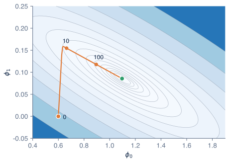
Figure 5.1 Gradient descent on the loss map. The orange path starts at $\phi_0 = 0.6$, $\phi_1 = 0$ (loss 0.839) and follows equation 5.2 with learning rate $\alpha = 0.015$. The numbers mark the parameters after 10 steps (loss 0.0548) and 100 steps (loss 0.0123). After 1000 steps the path reaches the best line (green), with loss 0.00063.

The path has two phases, and both come from the shape of the map. The first step changes mostly $\phi_1$, because the loss is much more sensitive to the slope than to the intercept: the slope is multiplied by years up to 9. This takes the path quickly into the valley. On the valley floor the ground is almost level, the derivatives are small, and so the steps are small too. Getting from step 10 to the bottom takes most of the 1000 steps.

2. The learning rate

The learning rate trades speed against stability. A one-parameter example makes this exact. Take the loss $L(\phi) = (\phi - 3)^2$, whose lowest point is at $\phi = 3$, and whose derivative is $2(\phi - 3)$. One step of gradient descent gives:

$$\phi \leftarrow \phi - \alpha \cdot 2(\phi - 3) \quad\text{which means}\quad \phi_{\text{new}} - 3 = (1 - 2\alpha)(\phi - 3)$$

Every step multiplies the distance to the minimum by $1 - 2\alpha$. Starting from $\phi = 0$ (figure 5.2):

• With $\alpha = 0.05$, the factor is 0.9. Each step removes only a tenth of the remaining distance, and after 8 steps $\phi$ has reached only 1.709.
• With $\alpha = 0.3$, the factor is 0.4, and after 8 steps $\phi = 2.998$.
• With $\alpha = 1.02$, the factor is $-1.04$. Each step jumps past the minimum to the other side, and lands slightly farther away than before: $6.12$, then $-0.245$, then $6.375$, and so on. Training diverges.

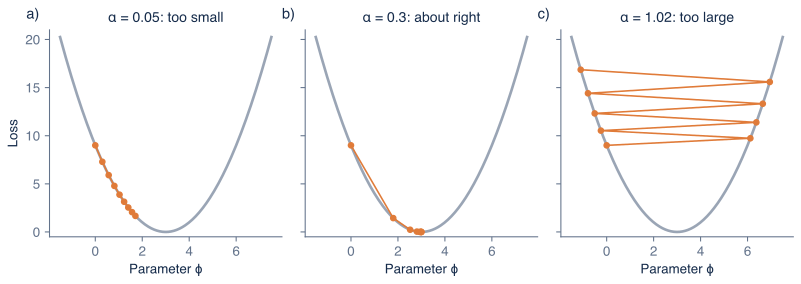
Figure 5.2 The learning rate. Eight steps of gradient descent on the loss $(\phi - 3)^2$, starting from $\phi = 0$. a) $\alpha = 0.05$: the steps are safe but slow. b) $\alpha = 0.3$: the parameter reaches the minimum quickly. c) $\alpha = 1.02$: every step overshoots, and the parameter moves farther from the minimum each time.

Real loss maps are not this simple, and no formula gives the best learning rate. In practice, people try several values and keep the one whose model performs best on a validation set (article 6).

The same trade-off appears when training a network. The experiment below trains a network with four hidden units to separate an inner cluster of points from a ring around it, starting with $\alpha = 0.003$.

Press play and watch the training loss above the output. With a learning rate of 0.003 it falls slowly: after 100 epochs it is still above 0.3. Set Learning rate to 0.03 and press the reset button (↺, left of play) to start training again. Now the loss is below 0.06 by epoch 100. Then set it to 10 and reset again. Within a few epochs the loss jumps above its starting value and never comes back down: every step overshoots, as in figure 5.2c, and the network ends up stuck far from a good fit.

Open in TensorFlow Playground ↗

3. When the lowest point is hard to reach

Gradient descent finds the bottom of the line's loss map because that map is a single bowl. Two things can still go wrong in general.

The model may be poorly chosen. Training can only find the lowest point the model family allows. If we replace the line with a model that predicts the same price every year, its best possible loss on the house data is 0.0612, about a hundred times the line's 0.00063. No training method can fix this, because no constant fits a rising trend. A poorly designed model has a high lowest point. The reverse problem, a model so flexible that it fits the noise in the training data, is the subject of article 6.

The map may have several valleys. The loss map of a neural network is not a bowl. It can have many valleys of different depths, plus flat plateaus. Gradient descent only ever walks downhill, so it stops at the bottom of whichever valley it walks into, which is called a local minimum. Where it starts decides which valley that is (figure 5.3).

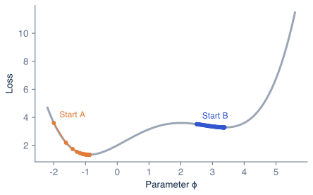
Figure 5.3 The starting point matters. A loss with two valleys. Gradient descent from start A ($\phi = -2.0$, orange) reaches the deeper valley at $\phi = -0.886$, with loss 1.333. From start B ($\phi = 2.5$, blue), the same algorithm stops in the shallower valley at $\phi = 3.376$, with loss 3.282, because every direction out of that valley goes uphill.

The starting parameters are chosen at random, a step called initialization. Besides deciding which valley training ends up in, the scale of the random values matters a great deal in deep networks. If the initial weights are too large, the values passing through the network grow from layer to layer until they overflow. If they are too small, the values shrink towards zero. In both cases the derivatives that guide training become useless, and training stalls. Standard schemes choose the scale from the number of inputs to each unit. For ReLU networks, He initialization [3] draws each weight from a distribution with variance $2 / D_{\text{in}}$, where $D_{\text{in}}$ is the number of inputs to the unit.

One-dimensional pictures like figure 5.3 can exaggerate the danger of local minima. In networks with millions of parameters, there is usually some direction that still goes downhill, and many of the valleys that training reaches have similar losses [6]. Poor initialization and a poor learning rate are more common causes of failed training than unlucky valleys.

4. Computing the gradient for a network

Equation 5.1 was easy to derive because a line is simple. A network has many layers, and each parameter affects the loss through every layer after it. The algorithm that computes all the derivatives efficiently is called backpropagation [2]. It is the chain rule of calculus applied systematically: the effect of a parameter on the loss is the product of its effects along the way.

We work through the smallest case: one input, one hidden unit with ReLU, and one output:

$$h = \mathrm{ReLU}(\theta_0 + \theta_1 x), \qquad f = \phi_0 + \phi_1 h, \qquad \ell = (f - y)^2 \tag{5.3}$$

where $\ell$ is the squared error for a single training example. We take the parameters $\theta_0 = 0$, $\theta_1 = 1$, $\phi_0 = 0$, $\phi_1 = 2$ and the example $x = 1.5$, $y = 2$.

The forward pass computes the values from input to loss. The pre-activation is $0 + 1 \times 1.5 = 1.5$, which is positive, so $h = 1.5$. The prediction is $f = 0 + 2 \times 1.5 = 3$, and the loss is $\ell = (3 - 2)^2 = 1$.

The backward pass computes the derivatives from the loss back towards the input, reusing each result for the next:

1. How the loss depends on the prediction: $\partial \ell / \partial f = 2(f - y) = 2$.
2. The output parameters: $f$ grows by 1 when $\phi_0$ grows by 1, so $\partial \ell / \partial \phi_0 = 2$. It grows by $h = 1.5$ when $\phi_1$ grows by 1, so $\partial \ell / \partial \phi_1 = 2 \times 1.5 = 3$.
3. The hidden unit: $f$ grows by $\phi_1 = 2$ per unit of $h$, so $\partial \ell / \partial h = 2 \times 2 = 4$.
4. Through the ReLU: the pre-activation is positive, so ReLU passes changes through unchanged (slope 1), and the derivative with respect to the pre-activation is also 4.
5. The first-layer parameters: $\partial \ell / \partial \theta_0 = 4 \times 1 = 4$ and $\partial \ell / \partial \theta_1 = 4 \times x = 6$.

Every derivative here can be checked by nudging the parameter by a tiny amount and recomputing the loss. Backpropagation gets all of them in one backward pass that costs about as much as the forward pass, however many parameters there are. Deep learning libraries do this automatically, which is why we rarely write derivatives by hand.

5. Training on large datasets

Equation 5.1 sums over all $I$ training examples. With a million photographs, every single step would need a million forward and backward passes. Stochastic gradient descent (SGD) instead computes the gradient on a small random subset of the training data, called a batch or mini-batch, often 32 to 512 examples, and takes a step after each batch. The gradient from a batch is a noisy estimate of the full gradient, but it costs a tiny fraction as much. One pass through the whole training set is called an epoch, and training usually runs for many epochs.

Improved versions of SGD are now standard. Momentum lets each step continue partly in the direction of the previous steps, which speeds up progress along long valleys like the one in figure 5.1. Adam [5] also adapts the step size separately for each parameter.

Putting the pieces together gives the training loop used, with variations, for almost every neural network:

1. Initialize the parameters randomly, at a suitable scale.
2. Take a batch of training examples.
3. Forward pass: compute the predictions and the loss.
4. Backward pass: compute the gradient by backpropagation.
5. Update the parameters with gradient descent or one of its variants.
6. Repeat from step 2, checking the performance on a validation set from time to time (article 6), and stop when it no longer improves.

Summary

Training searches the loss map for low points. Gradient descent computes the gradient, which points uphill, and takes a step of size set by the learning rate in the opposite direction. A learning rate that is too small makes training slow, and one that is too large makes it bounce or diverge. A poorly chosen model has a high lowest point. Gradient descent can stop in a local minimum, and the scale of the initial parameters decides whether deep networks train at all. Backpropagation computes all the derivatives of a network efficiently with the chain rule, and stochastic gradient descent makes each step cheap by using small batches.

Notes

Rescaling the inputs. The valley in figure 5.1 is long and narrow because the year takes values up to 9 while the intercept multiplies 1. If we measure years from the middle of the data, so that they run from $-4.5$ to $4.5$, the valley becomes much rounder and gradient descent converges in far fewer steps. This is why inputs are usually normalized to similar ranges before training.

Saddle points. In many dimensions, a point where the gradient is zero is more often a saddle point, downhill in some directions and uphill in others, than a true local minimum. Gradient descent slows down near saddle points but usually escapes them [6].

Initialization history. Glorot and Bengio [4] analysed how the scale of initial weights affects the values flowing through deep networks with sigmoid and tanh activations; He and colleagues [3] adapted the analysis to ReLU.

Reading further. Chapters 6 and 7 of Understanding Deep Learning [1] cover gradient descent, SGD, momentum, Adam, backpropagation and initialization.

Problems

Problem 5.1 For the loss $(\phi - 3)^2$, which learning rate reaches the minimum in exactly one step from any starting point? (Answer: $\alpha = 0.5$, which makes the factor $1 - 2\alpha$ zero.)

Problem 5.2 In the backpropagation example, what are the five derivatives if the example is $x = -1$ instead, with $y = 2$? (Answer: the pre-activation is $-1$, so $h = 0$, $f = 0$ and $\partial \ell / \partial f = -4$; then $\partial \ell / \partial \phi_0 = -4$, $\partial \ell / \partial \phi_1 = 0$, and both $\theta$ derivatives are 0 because the ReLU is off.)

Problem 5.3 A training set has 50,000 images and the batch size is 100. How many parameter updates make up one epoch? (Answer: 500.)

References

• 1: Simon J.D. Prince (2023). Understanding Deep Learning. MIT Press.
• 2: David Rumelhart, Geoffrey Hinton and Ronald Williams (1986). Learning representations by back-propagating errors. Nature 323, 533–536.
• 3: Kaiming He, Xiangyu Zhang, Shaoqing Ren and Jian Sun (2015). Delving deep into rectifiers: surpassing human-level performance on ImageNet classification. International Conference on Computer Vision.
• 4: Xavier Glorot and Yoshua Bengio (2010). Understanding the difficulty of training deep feedforward neural networks. International Conference on Artificial Intelligence and Statistics.
• 5: Diederik Kingma and Jimmy Ba (2015). Adam: a method for stochastic optimization. International Conference on Learning Representations.
• 6: Yann Dauphin, Razvan Pascanu, Caglar Gulcehre, Kyunghyun Cho, Surya Ganguli and Yoshua Bengio (2014). Identifying and attacking the saddle point problem in high-dimensional non-convex optimization. Advances in Neural Information Processing Systems 27.