Loss functions: measuring how wrong a model is

Articles 1 and 3 described models as families of functions: every choice of parameters gives a different line or a different network. To learn from data, we need to say which choice is better, and "better" must be a number a computer can compare. A loss function provides that number: it takes the model's predictions on the training data and returns a single value that is small when the predictions are good and large when they are bad. This article builds the loss for predicting numbers, draws it as a map over the parameters, and then builds the loss for predicting categories.

1. Measuring how far a line is from the data

We return to the house prices of article 1. Figure 4.1 shows three candidate lines. The first predicts the same price, 1.45, every year. The second rises too steeply. The third follows the data closely. We can see which is best, but we need a rule that a computer can apply.

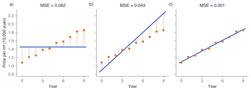
Figure 4.1 Three lines and their errors. Each panel shows the house-price data (orange) and one line $y = \phi_0 + \phi_1 x$ (blue). The dotted segments are the errors: the vertical distance between each data point and the line. a) $\phi_0 = 1.45$, $\phi_1 = 0$: a flat line, mean squared error 0.0622. b) $\phi_0 = 0.9$, $\phi_1 = 0.15$: too steep, 0.0434. c) $\phi_0 = 1.096$, $\phi_1 = 0.0857$: the best line, 0.00063.

The rule starts from the error for each example: the difference between the prediction $f(x_i, \boldsymbol{\phi})$ and the true value $y_i$. These are the dotted segments in figure 4.1. To combine the ten errors into one number, we square each one and take the average:

$$L(\boldsymbol{\phi}) = \frac{1}{I} \sum_{i=1}^{I} \big( f(x_i, \boldsymbol{\phi}) - y_i \big)^2 \tag{4.1}$$

We can break this down into three steps. First, for each training example $i$, we compute the prediction and subtract the true value. Second, we square the result. Finally, we add the squares for all $I$ examples and divide by $I$. This is the mean squared error, or MSE. In words: the MSE is the average squared distance between the predictions and the truth.

For the flat line in figure 4.1a, the prediction is 1.45 every year. In year 0 the true price is 1.08, so the error is $0.37$ and its square is $0.1369$. In year 9 the true price is 1.85, the error is $-0.40$ and its square is $0.16$. The ten squares add up to $0.6224$, and dividing by $I = 10$ gives $L = 0.0622$. The same calculation gives $0.0434$ for the steep line and $0.00063$ for the line that follows the data.

Squaring does two things. It makes every error count positively, so that errors above and below the line cannot cancel. It also makes large errors count much more than small ones: an error of 0.4 adds 16 times as much to the loss as an error of 0.1. Sometimes that is undesirable, for example when a few data points are wrong records. The mean absolute error, which averages $|f(x_i, \boldsymbol{\phi}) - y_i|$ instead, is less affected by such points.

2. The loss map

The loss depends on the parameters. For our line there are only two, $\phi_0$ and $\phi_1$, so we can compute the loss for every combination and draw it as a map (figure 4.2). Each point on the map is one line, and its colour is that line's loss.

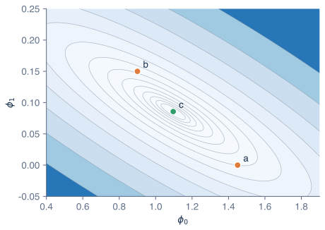
Figure 4.2 The loss map for the house-price line. Every point $(\phi_0, \phi_1)$ is one line, and its shading shows the mean squared error of that line on the ten data points; darker blue means larger loss. Gray curves connect lines with equal loss. Points a and b (orange) are the lines of figures 4.1a and 4.1b. Point c (green) is the line of figure 4.1c, at the lowest point of the map.

Training a model means finding the lowest point on this map. For a line we can see it directly; it is the green point c. The map also shows something less obvious: the low region is a long, narrow valley running diagonally. Raising the slope $\phi_1$ while lowering the intercept $\phi_0$ keeps the line passing near the middle of the data, so many such pairs have similar losses. Article 5 shows that the shape of this valley affects how quickly training finds the bottom.

A network with millions of parameters has a loss map with millions of dimensions, which nobody can draw. The principle does not change: the loss assigns a number to every choice of parameters, and training searches for a choice with a low number. This picture is often called the loss landscape or loss surface.

3. Predicting categories

For classification, the output is a category such as "cat", "dog" or "other", and the squared difference between categories means nothing. Instead, we let the network output one number per category and turn those numbers into probabilities.

Suppose a network looks at a photograph and outputs the scores $z_1 = 2.0$ for cat, $z_2 = 0.5$ for dog and $z_3 = -1.0$ for other. The scores can be any numbers, positive or negative. The softmax function turns them into probabilities:

$$p_k = \frac{e^{z_k}}{\sum_{j=1}^{K} e^{z_j}} \tag{4.2}$$

Here $K$ is the number of categories and $e^{z}$ is the exponential function. We can break this down into two steps. First, exponentiating makes every score positive while keeping their order: $e^{2.0} = 7.389$, $e^{0.5} = 1.649$ and $e^{-1.0} = 0.368$. Second, dividing by their sum, $9.406$, makes them add up to 1. The probabilities are $p_1 = 0.786$, $p_2 = 0.175$ and $p_3 = 0.039$ (figure 4.3a–b). In words: softmax turns scores into probabilities, and a higher score always means a higher probability.

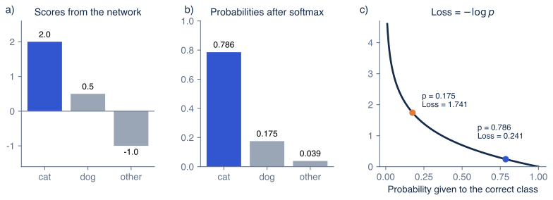
Figure 4.3 From scores to a classification loss. a) The network's scores for three categories. b) Softmax (equation 4.2) turns them into probabilities that add up to 1. c) The cross-entropy loss $-\log p$, where $p$ is the probability given to the correct category. If the photograph shows a cat, $p = 0.786$ and the loss is 0.241 (blue). If it shows a dog, $p = 0.175$ and the loss is 1.741 (orange).

4. The cross-entropy loss

A good classifier should give a high probability to the correct category. The cross-entropy loss measures this with a logarithm:

$$L = -\log p_c \tag{4.3}$$

where $p_c$ is the probability the model gives to the correct category $c$, and $\log$ is the natural logarithm. Over a training set, we average this quantity over all the examples, just as the MSE averages over examples.

Figure 4.3c shows how this loss behaves. If the photograph really shows a cat, the loss is $-\log 0.786 = 0.241$. If it shows a dog, the model gave the right answer only probability 0.175 and the loss is $-\log 0.175 = 1.741$. If it shows neither, the loss is $-\log 0.039 = 3.241$. When the correct probability approaches 1, the loss approaches 0. When it approaches 0, the loss grows without limit. A model that is confident and wrong is therefore punished much more than one that is unsure.

When there are only two categories, such as spam and not spam, the network often outputs a single score $z$ and converts it with the sigmoid function $p = 1 / (1 + e^{-z})$ into the probability of the first category. The loss is then $-\log p$ for examples of the first category and $-\log(1 - p)$ for the others. This is called the binary cross-entropy, and it is the special case of equation 4.3 for two categories.

5. Choosing a loss

The loss follows from the type of output:

Task	Output	Usual loss
Regression (price, temperature)	A number	Mean squared error, or mean absolute error
Binary classification (spam or not)	One probability	Binary cross-entropy
Multi-class classification (cat, dog, other)	One probability per class	Cross-entropy after softmax
Object detection	Boxes and labels	A box error, such as absolute error on coordinates, plus cross-entropy for the label
Segmentation	A label per pixel	Cross-entropy for each pixel, averaged over pixels

A loss is used for training, so it must change smoothly when the parameters change slightly; article 5 explains why. This is why we train classifiers with cross-entropy rather than with the percentage of correct answers. The percentage of correct answers jumps from one value to another and gives no signal about which direction to move the parameters. We still use percentages and similar metrics to report how good a model is, and article 6 covers them.

Summary

A loss function turns a model's predictions on the training data into one number that measures how wrong they are. For predicting numbers, the mean squared error averages the squared differences between predictions and true values. Because the loss depends on the parameters, it can be drawn as a map, and training means finding its lowest point. For predicting categories, softmax turns the network's scores into probabilities, and the cross-entropy loss is the negative logarithm of the probability given to the correct category.

Notes

Why these losses. The mean squared error and the cross-entropy both follow from one principle, maximum likelihood: choose the parameters that make the observed training data most probable. Assuming the errors follow a normal (Gaussian) distribution leads to the mean squared error, and treating the output as a probability for each category leads to the cross-entropy. Chapter 5 of Understanding Deep Learning [1] develops this recipe and uses it to build losses for other kinds of output.

Sum or mean. Some books define the squared-error loss as the sum over examples rather than the mean. The two differ only by the constant factor $I$, so they have the same lowest point.

Scores and probabilities. The scores before softmax are often called logits. Adding the same constant to every score leaves the probabilities unchanged, so only the differences between scores matter.

Problems

Problem 4.1 A line predicts 1.50, 1.60 and 1.70 for three years whose true prices are 1.40, 1.65 and 1.70. What is its mean squared error? (Answer: $(0.01 + 0.0025 + 0)/3 \approx 0.00417$.)

Problem 4.2 A network outputs the scores $(1, 1, 1)$ for three categories. What probabilities does softmax give, and what is the cross-entropy loss for any correct category? (Answer: each probability is $1/3$, and the loss is $\log 3 \approx 1.099$.)

Problem 4.3 Explain why the loss in equation 4.3 cannot be negative.

References

• 1: Simon J.D. Prince (2023). Understanding Deep Learning. MIT Press.