Neural networks: functions that can bend

The straight line of article 1 has two parameters and one shape: it can only describe a relationship that changes at a constant rate. Article 2 showed the other limitation of traditional methods, that their features must be designed by hand. This article introduces neural networks, a family of functions that can bend into almost any shape and that grow naturally from one input to millions. We build the smallest interesting network by hand, see what it can represent, and then generalise it.

1. A network with three hidden units

We start with a network that maps one input $x$ to one output $y$, like the house-price line. We defer the general definition until section 3. The network computes three intermediate values $h_1$, $h_2$ and $h_3$, and then combines them:

$$\begin{aligned} h_1 &= a(\theta_{10} + \theta_{11} x) \\ h_2 &= a(\theta_{20} + \theta_{21} x) \\ h_3 &= a(\theta_{30} + \theta_{31} x) \end{aligned} \tag{3.1}$$ $$y = \phi_0 + \phi_1 h_1 + \phi_2 h_2 + \phi_3 h_3 \tag{3.2}$$

We can break the computation into three steps. First, we compute three different linear functions of the input, $\theta_{10} + \theta_{11} x$ and so on, each with its own offset and slope. Second, we pass each result through a function $a(\cdot)$. Finally, we multiply the three results by $\phi_1$, $\phi_2$ and $\phi_3$, add them up and add an offset $\phi_0$. The network has ten parameters: six $\theta$s ("theta") and four $\phi$s.

To complete the description, we must define $a(\cdot)$, which is called the activation function. The most common choice is the rectified linear unit, or ReLU:

$$a(z) = \mathrm{ReLU}(z) = \max(0, z) = \begin{cases} 0 & z < 0 \\ z & z \ge 0 \end{cases} \tag{3.3}$$

In words, ReLU passes positive values through unchanged and replaces negative values with zero.

To see the network in action, we choose values for the ten parameters:

	Offset	Slope	Output weight
Unit 1	$\theta_{10} = -0.4$	$\theta_{11} = 1.0$	$\phi_1 = 1.0$
Unit 2	$\theta_{20} = 1.0$	$\theta_{21} = -1.0$	$\phi_2 = -0.8$
Unit 3	$\theta_{30} = -1.8$	$\theta_{31} = 1.2$	$\phi_3 = -1.5$

with output offset $\phi_0 = 0.2$. For the input $x = 1.2$, the three linear functions give $-0.4 + 1.2 = 0.8$, then $1.0 - 1.2 = -0.2$, then $-1.8 + 1.2 \times 1.2 = -0.36$. ReLU keeps the first and sets the other two to zero, so $h_1 = 0.8$ and $h_2 = h_3 = 0$. The output is:

$$y = 0.2 + 1.0 \times 0.8 + (-0.8) \times 0 + (-1.5) \times 0 = 1.0$$

Figure 3.1 repeats this computation for every input between 0 and 2.

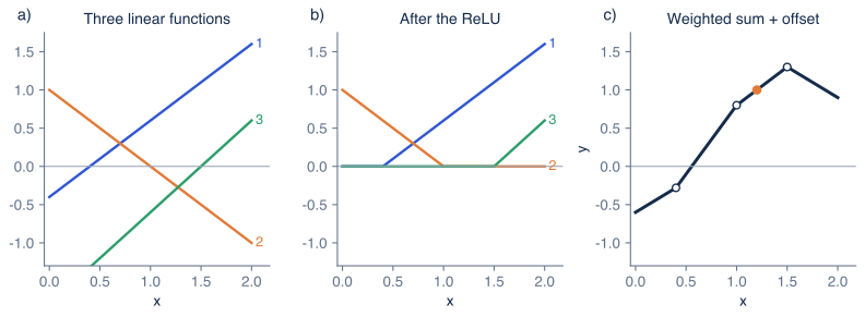
Figure 3.1 How the network builds its output. a) The three linear functions $\theta_{d0} + \theta_{d1} x$ for $d = 1, 2, 3$ (blue, orange, green). b) After the ReLU, each is zero wherever it was negative. c) The output $y$ of equation 3.2 is a weighted sum of the three curves in (b), plus $\phi_0$. It consists of straight segments joined at three corners (open circles), at $x = 0.4$, $1.0$ and $1.5$. The orange dot is the worked example $x = 1.2$, $y = 1.0$.

2. What the network can represent

Figure 3.1c shows the key property. The output is still made of straight pieces, but unlike a single line it can change direction. Each hidden unit contributes one joint, where its linear function crosses zero and ReLU switches between "off" and "on". For unit $d$, this happens where $\theta_{d0} + \theta_{d1} x = 0$, that is, at $x = -\theta_{d0} / \theta_{d1}$. For our values the joints are at $0.4$, $1.0$ and $1.5$.

Between two joints, each unit is either off (contributing nothing) or on (contributing a straight line), so the output is a straight line there too. Its slope is the sum of the slopes of the units that are on. For $0.4 < x < 1.0$, units 1 and 2 are on, so the slope is $\phi_1 \theta_{11} + \phi_2 \theta_{21} = 1.0 \times 1.0 + (-0.8) \times (-1.0) = 1.8$. Past $x = 1.5$, units 1 and 3 are on and the slope is $1.0 - 1.5 \times 1.2 = -0.8$, so the output turns downward. Changing a unit's offset moves its joint left or right; changing its output weight changes how sharply the output bends there.

A function made of straight pieces like this is called piecewise linear. With three hidden units and one input, the network can make at most three joints and therefore at most four pieces. More hidden units allow more joints. Figure 3.2 shows networks with 3, 6 and 12 hidden units approximating a smooth curve. The largest gap between the network and the curve shrinks from 0.89 to 0.25 to 0.07.

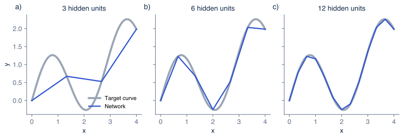
Figure 3.2 More hidden units, more flexibility. a–c) A network with 3, 6 and 12 hidden units (blue) approximating a smooth target curve (gray) between $x = 0$ and $x = 4$. Here the parameters were chosen by hand, so that the network's joints lie on the curve at evenly spaced points. With more units the straight pieces get shorter and the approximation gets closer.

This pattern holds in general. The universal approximation theorem [2], [3] says that a network with one hidden layer can approximate any continuous function on a bounded range of inputs as closely as we like, provided it has enough hidden units. The theorem is about what networks can represent. It does not say how many hidden units are needed, it does not say that training will find good parameters (article 5), and it does not say that the result will work well on new data (article 6).

3. Many inputs and many outputs

Real problems have more than one input. A house-price model might use the year, the floor area and the distance to the city centre. The extension is direct: each hidden unit now computes a weighted sum of all the inputs before applying the activation function. With inputs $x_1, \ldots, x_{D_i}$, hidden unit $d$ computes:

$$h_d = a\left(\theta_{d0} + \sum_{j=1}^{D_i} \theta_{dj} x_j\right) \tag{3.4}$$

If there are several outputs, each output $y_k$ has its own weights for combining the hidden units:

$$y_k = \phi_{k0} + \sum_{d=1}^{D} \phi_{kd} h_d \tag{3.5}$$

Here $D_i$ is the number of inputs, $D$ the number of hidden units and $D_o$ the number of outputs. With one input, three hidden units and one output, equations 3.4 and 3.5 reduce to equations 3.1 and 3.2.

Counting parameters is a useful check. Each hidden unit has one offset and $D_i$ input weights, and each output has one offset and $D$ weights, so the total is:

$$D(D_i + 1) + D_o(D + 1)$$

Our first network has $3 \times 2 + 1 \times 4 = 10$ parameters, as counted before. A house-price network with 3 inputs, 4 hidden units and 1 output has $4 \times 4 + 1 \times 5 = 21$. Feeding the 135,300 pixels of the cat photograph into 100 hidden units with 3 outputs needs 13,530,403 parameters, which is one reason images use the convolutional networks mentioned in article 2.

Written with vectors and matrices, equations 3.4 and 3.5 become $\mathbf{h} = a(\boldsymbol{\theta}_0 + \boldsymbol{\Theta}\mathbf{x})$ and $\mathbf{y} = \boldsymbol{\phi}_0 + \boldsymbol{\Phi}\mathbf{h}$, where $a$ is applied to each element separately. This is the same computation in compact form; the notation page explains the symbols.

4. Deep networks

The network so far has a single hidden layer: one set of hidden units between input and output. A deep network has several, and each layer takes the previous layer's outputs as its inputs (figure 3.3). The second layer computes new linear functions of $h_1, h_2, h_3$ and applies the activation function again, and so on.

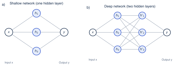
Figure 3.3 Shallow and deep networks. a) The network of section 1: one input, one hidden layer of three units, one output. Each line carries a weight. b) A deep network with two hidden layers. The second layer ($h'_1, h'_2, h'_3$) receives the outputs of the first layer as its inputs.

With ReLU activations, a deep network is still piecewise linear, but stacking layers lets it create joints far more economically. The second layer can fold and combine the pieces made by the first, so the number of linear pieces can grow much faster with depth than with width [4]. For many functions met in practice, deep networks reach a given accuracy with fewer parameters than shallow ones, and they are usually easier to train well. That is why nearly all modern networks are deep.

5. Why the activation function matters

Without an activation function, depth adds nothing. Suppose two layers are purely linear: $h = 2x + 1$ and then $y = 3h - 2$. Substituting the first into the second gives:

$$y = 3(2x + 1) - 2 = 6x + 1$$

The two layers are exactly equivalent to one straight line. The same holds for any number of linear layers with any number of units: substituting one into the next always produces another linear function. A deep network without activation functions can represent nothing that a single linear layer could not.

Putting ReLU between the layers breaks the substitution. The function $y = 3 \, \mathrm{ReLU}(2x + 1) - 2$ equals $-2$ for $x \le -0.5$ and $6x + 1$ for larger $x$: it has a corner, and no single line can describe it. The activation function is what lets a network bend, and stacking bends is what makes depth useful.

The same effect is easy to see in two dimensions. In the experiment below, a network with three hidden ReLU units, as in section 1 but with two inputs, learns to separate an inner cluster of points from a ring around it.

Press play. Each hidden unit computes a ramp with one straight crease; hover a unit to see it. Within about a hundred epochs, the three creases combine into a closed, angular region around the inner cluster. Then set Activation to Linear. The network resets; train it again. However long it runs, the boundary stays a straight line and the loss stops falling, because linear units add up to one linear function.

Open in TensorFlow Playground ↗

6. Terminology

Now that we have seen how a network computes, we can name its parts.

• The input layer holds the inputs $x$. The output layer produces $y$. The layers in between are hidden layers, because their values are never observed in the training data.
• The intermediate values $h_d$ are hidden units, also called neurons. The values before the activation function, such as $\theta_{10} + \theta_{11} x$, are pre-activations, and the values after it are activations.
• The slopes ($\theta_{11}$, $\phi_1$, …) are weights, and the offsets ($\theta_{10}$, $\phi_0$, …) are biases.
• The number of hidden units in a layer is its width, and the number of hidden layers is the network's depth.
• A network in which every unit of one layer connects to every unit of the next is fully connected. The networks in this article are of this kind, and are also called multilayer perceptrons.

Summary

A neural network computes linear functions of its inputs, passes them through an activation function such as ReLU, and combines the results linearly. With ReLU, each hidden unit adds a joint, so the network describes piecewise linear functions, and with enough hidden units it can approximate any continuous function. The idea extends directly to many inputs and outputs and to many layers. Without activation functions, any stack of layers collapses to a single linear function. We now have a flexible family of functions; article 4 defines how to measure which member of it fits the data best.

Notes

Other activation functions. Early networks used the sigmoid $1/(1 + e^{-z})$ and $\tanh$. ReLU [5] became the default because it is cheap to compute and because its slope does not shrink towards zero for large positive inputs, which makes deep networks easier to train. Newer variants such as GELU are smooth near zero; with them the network is no longer exactly piecewise linear, but the picture of this article still describes it well.

Same function, different training. Two stacked linear layers represent the same functions as one, but they are not identical during training: the product of two weight matrices changes differently under gradient descent than a single matrix. This matters in research on how networks learn, but it does not add new functions.

"Neurons". The name comes from a loose analogy with nerve cells, which receive many inputs and fire when stimulated enough. Modern networks are not models of the brain, and the analogy does not explain why they work.

Reading further. Chapters 3 and 4 of Understanding Deep Learning [1] treat shallow and deep networks in more depth, including how to count the linear regions.

Problems

Problem 3.1 Using the parameter values of section 1, compute $y$ for $x = 0$ and for $x = 2$. (Answer: $-0.6$ and $0.9$.)

Problem 3.2 How many parameters does a fully connected network have with 10 inputs, one hidden layer of 20 units and 2 outputs? (Answer: $20 \times 11 + 2 \times 21 = 262$.)

Problem 3.3 A network has three linear layers and no activation functions: $h = 2x$, $h' = h - 1$, $y = -3h' + 4$. Write $y$ as a single linear function of $x$. (Answer: $y = -6x + 7$.)

References

• 1: Simon J.D. Prince (2023). Understanding Deep Learning. MIT Press.
• 2: Kurt Hornik, Maxwell Stinchcombe and Halbert White (1989). Multilayer feedforward networks are universal approximators. Neural Networks 2(5), 359–366.
• 3: Moshe Leshno, Vladimir Lin, Allan Pinkus and Shimon Schocken (1993). Multilayer feedforward networks with a nonpolynomial activation function can approximate any function. Neural Networks 6(6), 861–867.
• 4: Guido Montúfar, Razvan Pascanu, Kyunghyun Cho and Yoshua Bengio (2014). On the number of linear regions of deep neural networks. Advances in Neural Information Processing Systems 27.
• 5: Vinod Nair and Geoffrey Hinton (2010). Rectified linear units improve restricted Boltzmann machines. International Conference on Machine Learning.