Features: turning raw data into useful numbers

Article 1 explained that traditional machine learning depends on hand-designed features. This article shows what a feature is and how some classic image features are computed, one multiplication at a time. Seeing how much design goes into them also shows what deep learning saves us from designing.

1. What a feature is

A feature is a number computed from raw data that re-expresses it in a form that makes a task easier. Raw data is whatever we record directly: every individual house sale, every pixel of a photograph, every word of a message. Features summarise or transform it.

The house prices in article 1 were already a feature. The raw data would be thousands of individual sales, each with a price, a floor area and a date. We reduced each year to one number, the average price per square metre. Other features of the same data could be useful too: the variance of the prices, which measures how spread out they are, or the number of sales each year, which measures how active the market is.

Text gives another example. Suppose we want to tell spam from ordinary email. A simple feature is the number of times each of a few chosen words appears:

Message	"free"	"winner"	"prize"	"meeting"	"notes"
"Congratulations, you are a winner! Claim your free prize now."	1	1	1	0	0
"Can we move the meeting to Friday? I will send the notes."	0	0	0	1	1

Each message becomes a list of five numbers, a feature vector. A learning algorithm never sees the sentences, only these vectors, so it can only learn what the vectors preserve. If the spammer writes "fr3e" instead of "free", this feature misses it. Choosing features means deciding in advance what information the model is allowed to use.

2. Images are grids of numbers

A grayscale image is a grid of numbers, one per pixel, usually from 0 (black) to 255 (white). Figure 2.1 zooms into an $8 \times 8$ patch of the cat photograph from article 1, where the bright fur meets the dark rim of the eye. The numbers fall from around 150 on the left to under 30 on the right. A colour image stores three such grids, for red, green and blue.

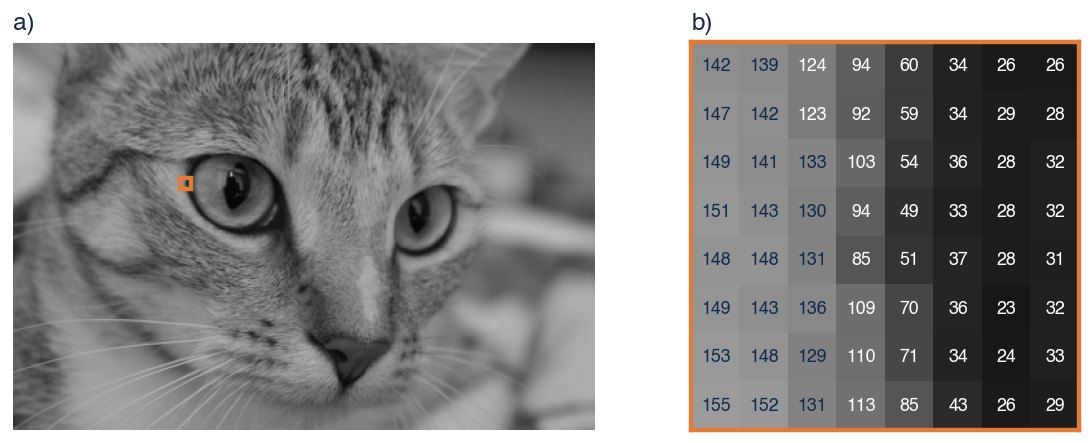
Figure 2.1 An image is a grid of numbers. a) The cat photograph in grayscale ($300 \times 451$ pixels). The orange square marks an $8 \times 8$ patch at the edge of the left eye. b) The patch enlarged, with the value of each pixel from 0 (black) to 255 (white). Brightness drops sharply from left to right where the fur meets the rim of the eye.

A person sees a cat in figure 2.1a at a glance. A computer receives 135,300 numbers. Image features try to compute, from those numbers, quantities that relate more directly to what the image shows, such as where its edges are.

3. Filtering with a small kernel

Many classic image features come from one operation: slide a small grid of weights, called a kernel, across the image, and at each position compute a weighted sum of the pixels underneath. We start with a single position and a $3 \times 3$ kernel, and extend to the whole image afterwards.

Take the $3 \times 3$ window in rows 3–5 and columns 3–5 of the patch in figure 2.1b:

$$W = \begin{bmatrix} 133 & 103 & 54 \\ 130 & 94 & 49 \\ 131 & 85 & 51 \end{bmatrix}$$

and a kernel $K$ of the same size. The filter output at this position is:

$$g = \sum_{m=1}^{3} \sum_{n=1}^{3} K_{mn} \, W_{mn} \tag{2.1}$$

The symbol $\sum$ means "add up". Equation 2.1 says: multiply each pixel by the kernel weight at the same position, then add the nine products. The kernel decides what the output measures. We try two kernels.

An averaging kernel. If every weight is $1/9$, the output is the mean of the nine pixels:

$$g = \frac{133 + 103 + 54 + 130 + 94 + 49 + 131 + 85 + 51}{9} = \frac{830}{9} \approx 92.2$$

The average smooths away differences between neighbouring pixels.

An edge kernel. The Sobel kernel for left–right changes is:

$$K_x = \begin{bmatrix} -1 & 0 & 1 \\ -2 & 0 & 2 \\ -1 & 0 & 1 \end{bmatrix}$$

It subtracts the left column from the right column, counting the middle row twice. For our window, the left column contributes $-133 - 2 \times 130 - 131 = -524$, the right column contributes $54 + 2 \times 49 + 51 = 203$, and the middle column contributes nothing, so:

$$g = -524 + 203 = -321$$

The large negative value says that brightness falls steeply from left to right, as it does at the rim of the eye. For comparison, the window in rows 1–3 and columns 6–8 lies inside the dark region, where all pixels are similar; there the same kernel gives only $-24$. The size of the output measures how strong the edge is, and its sign says which side is brighter.

Sliding the kernel to every position in the image and writing each output at that position produces a new image, sometimes called a feature map. This sliding weighted sum is called convolution. Strictly, equation 2.1 is a cross-correlation: mathematical convolution flips the kernel first. Deep learning libraries also use the unflipped version but still call it convolution.

4. A gallery of classic filters

Figure 2.2 applies several classic filters to the whole photograph. Each keeps some information and throws the rest away.

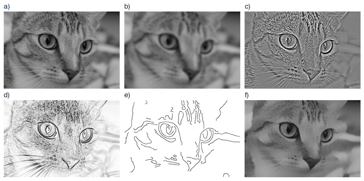
Figure 2.2 Classic image filters. a) The original grayscale image. b) Low-pass: a Gaussian blur with a width of 3 pixels keeps the slow changes in brightness and removes fine detail. c) High-pass: subtracting (b) from (a) keeps only the fine detail, such as fur and whiskers. d) Edge strength from the Sobel kernels; darker means a stronger edge. e) Canny edges: thin, connected edge curves. f) Bilateral filter: smooths the fur while keeping the edges of the eyes and nose sharp.

• Low-pass filters (figure 2.2b) average each pixel with its neighbours, as our averaging kernel did. A Gaussian blur gives nearby pixels more weight than distant ones. The result keeps the large shapes and removes fine detail and noise.
• High-pass filters (figure 2.2c) do the opposite. One way is to subtract the low-pass image from the original, which leaves only what the blur removed: texture, whiskers, noise.
• Gradient filters (figure 2.2d) use Sobel kernels for left–right changes and up–down changes and combine the two outputs into an edge strength at every pixel.
• The Canny edge detector [2] (figure 2.2e) is a multi-step procedure rather than a single kernel. It blurs the image, computes gradients, keeps only the pixels where the edge strength peaks across the edge, and then links them using two thresholds. The output is a clean set of edge curves.
• The bilateral filter [3] (figure 2.2f) averages each pixel with neighbours that are both nearby and similar in brightness. Across an edge the neighbours are dissimilar, so they get little weight, and the edge stays sharp while flat regions are smoothed. Because the weights depend on the image itself, this is not a convolution with a fixed kernel.

Every panel depended on choices we made: the blur width, the Canny thresholds, how similar two pixels must be for the bilateral filter. Different choices give visibly different results.

5. From filter outputs to an answer

Filter outputs are still images, and still large. Traditional pipelines summarised them further into compact descriptors. A well-known example is the histogram of oriented gradients (HOG) [4]. It divides the image into small cells and, in each cell, counts how much edge strength points in each of several directions. Another is SIFT [5], which describes the neighbourhood of distinctive points so that they can be matched between images. A classifier, such as the support vector machine from article 1, then learned to map these descriptors to labels.

These systems worked. HOG with a support vector machine was a standard way to detect pedestrians, for example. But each stage had been designed by a person who had to guess what information the final task would need.

6. The limits of designed features

Hand-designed features have three weaknesses. First, they have to be invented separately for each kind of data and often for each task; edge features for photographs say nothing about sound or text. Second, every one discards information, and what it discards cannot be recovered later. The Canny output in figure 2.2e has lost the texture of the fur, which might be exactly what distinguishes a tabby cat from a tiger. Third, their settings are tuned by hand, and good settings for one dataset may be poor for another.

Convolutional neural networks [6] keep the sliding weighted sum of section 3 but learn the kernel weights from training data, along with everything after them. When such a network is trained to classify photographs, the kernels in its first layer often end up resembling edge and colour detectors [7], similar to the filters people had designed. The kernels in later layers respond to increasingly complex patterns that nobody specified. Article 3 introduces the neural networks that make this possible; convolutional networks are covered in the next part of the course.

The difference between choosing features and learning them is easy to try on a small problem. In the experiment below, a model with no hidden units, only a weighted sum of its inputs, must separate an inner cluster of points from a ring around it.

Press play. The model can only add up X₁ and X₂ with weights, so its boundary is a straight line, and the loss stops falling at about 0.5: no straight line separates a disc from the ring around it. Then click X₁² and X₂² to feed them in as well. The model resets; train it again. Within about twenty epochs the boundary becomes a circle and the loss drops below 0.02, because X₁² + X₂² is the squared distance from the centre. Choosing those two features required knowing that the data are round. Article 3 shows a network with hidden units finding such shapes by itself.

Open in TensorFlow Playground ↗

Summary

A feature is a number computed from raw data that makes a task easier. Images are grids of numbers, and many classic image features come from sliding a small kernel across the image and taking weighted sums. An averaging kernel smooths, and a Sobel kernel responds to edges. Canny edges, bilateral filtering and descriptors like HOG build on these operations. All of them require human choices, and each discards information. Deep learning keeps the sliding-kernel computation but learns the kernels from data.

Notes

Convolution and frequency. "Low-pass" and "high-pass" come from signal processing. Smooth variations in brightness correspond to low spatial frequencies and fine detail to high frequencies; a blur removes the high frequencies.

Image borders. At the edge of the image, part of the kernel falls outside it. Common fixes are to pad the image with zeros, to repeat the border pixels, or to compute outputs only where the kernel fits, which makes the output slightly smaller.

Text features. Word counts are called a bag of words, because word order is ignored. A widely used refinement, TF-IDF, down-weights words that appear in almost every document. Modern language models instead learn their own representations of words.

Reading further. Chapter 10 of Understanding Deep Learning [1] explains convolutional networks, including how learned kernels are stacked.

Problems

Problem 2.1 Apply the averaging kernel and the Sobel kernel $K_x$ to the window in rows 1–3 and columns 1–3 of figure 2.1b. (Answer: the mean is $1240/9 \approx 137.8$, and the Sobel output is $-82$.)

Problem 2.2 Write down a $3 \times 3$ kernel that responds to up–down changes in brightness instead of left–right changes. (Hint: rotate $K_x$ by 90 degrees.)

Problem 2.3 A bilateral filter and a Gaussian blur are applied to a photograph of a black square on a white background. Describe how the square's edge looks after each filter.

References

• 1: Simon J.D. Prince (2023). Understanding Deep Learning. MIT Press.
• 2: John Canny (1986). A computational approach to edge detection. IEEE Transactions on Pattern Analysis and Machine Intelligence 8(6), 679–698.
• 3: Carlo Tomasi and Roberto Manduchi (1998). Bilateral filtering for gray and color images. International Conference on Computer Vision.
• 4: Navneet Dalal and Bill Triggs (2005). Histograms of oriented gradients for human detection. Conference on Computer Vision and Pattern Recognition.
• 5: David G. Lowe (2004). Distinctive image features from scale-invariant keypoints. International Journal of Computer Vision 60, 91–110.
• 6: Yann LeCun, Léon Bottou, Yoshua Bengio and Patrick Haffner (1998). Gradient-based learning applied to document recognition. Proceedings of the IEEE 86(11), 2278–2324.
• 7: Alex Krizhevsky, Ilya Sutskever and Geoffrey Hinton (2012). ImageNet classification with deep convolutional neural networks. Advances in Neural Information Processing Systems 25.