Machine learning: learning a function from examples

Most problems in machine learning ask for the same thing: a function that takes some input and returns the right output. This article makes that idea concrete with a small example. It then explains how learning a function from examples differs from writing one by hand, and why deep learning goes one step further than earlier methods. The articles that follow take each ingredient in turn: features, neural networks, loss functions, training and evaluation.

The course assumes school algebra and the idea of a function. Article 5 uses derivatives; it explains what it needs as it goes. The structure follows Simon Prince's Understanding Deep Learning [1], which is free to read online and is the natural next step after this course.

1. Inputs, outputs and models

Many different tasks share one shape: an input goes in, and an output should come out. Four examples show the range:

Task	Input	Output
Predicting house prices	The year	The average price per square metre that year
Image classification	A photograph	One label, such as "cat", "dog" or "other"
Object detection	A photograph	A box around each object, plus its label
Segmentation	A photograph	A label for every pixel

Figure 1.1 shows the three image tasks on the same photograph. They become harder from left to right. Classification gives one answer for the whole image. Detection must also say where the object is. Segmentation must decide, for each of the 135,300 pixels in this image, whether it belongs to the cat.

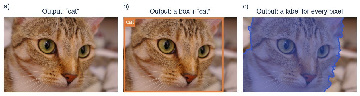
Figure 1.1 Three tasks on one image. a) Classification: the output is one label for the whole image. b) Object detection: the output is a box that encloses the object, plus a label. c) Segmentation: the output is a label for every pixel; here the shaded pixels are "cat" and the rest are "background". These are the outputs each task asks for, drawn by hand, not the predictions of a trained model. Photograph: scikit-image sample image "chelsea" (CC0).

In every case we want a function $f$ that maps the input $x$ to the output $y$:

$$y = f(x) \tag{1.1}$$

We call $f$ the model. Computing $y$ from a new input $x$ is called inference or prediction. The rest of this article looks at where $f$ comes from.

2. A first model: a straight line

Consider the average price of housing in a fictional city. We have one measurement per year for ten years (figure 1.2): the price per square metre rose from 1.08 to 1.85, measured in units of 10,000 yuan. We would like to predict the price in year 10, the year after the last measurement.

The simplest reasonable model is a straight line:

$$y = f(x, \boldsymbol{\phi}) = \phi_0 + \phi_1 x \tag{1.2}$$

Here $x$ is the year and $y$ is the predicted price. The two numbers $\phi_0$ and $\phi_1$ ("phi zero" and "phi one") are the parameters of the model, and we write them together as $\boldsymbol{\phi} = (\phi_0, \phi_1)$. The parameter $\phi_0$ is the height of the line at year 0, and $\phi_1$ is its slope: how much the price changes per year.

Equation 1.2 does not describe one line but a whole family of lines, one for each choice of $\phi_0$ and $\phi_1$. Choosing the parameters picks one member of the family. For this data, the line with $\phi_0 = 1.096$ and $\phi_1 = 0.0857$ passes close to every measurement (figure 1.2). Its prediction for year 10 is:

$$y = 1.096 + 0.0857 \times 10 = 1.953$$

That is, about 19,500 yuan per square metre.

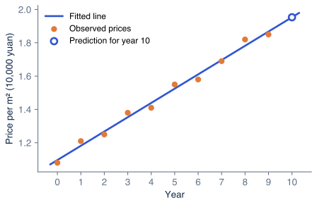
Figure 1.2 A straight-line model of house prices. The orange points are the average price per square metre in a fictional city for years 0 to 9. The blue line is equation 1.2 with $\phi_0 = 1.096$ and $\phi_1 = 0.0857$. Extending the line to year 10 gives the prediction 1.953 (open circle).

We have not yet said how those two numbers were found; that is the subject of articles 4 and 5. Two cautions apply already. First, the prediction assumes the trend of the last ten years continues, and nothing in the data guarantees that. Second, a line cannot bend, so if prices sped up or levelled off, this family of functions could not follow them. Article 3 introduces models that can bend.

3. Learning instead of writing rules

One way to build $f$ would be to write it by hand: an expert studies the market and writes down a formula. Machine learning takes a different route. We choose a family of functions, such as all straight lines, and let an algorithm choose the member of the family that best matches a set of examples. The examples are called the training data, and choosing the parameters from them is called training or learning.

When each training example comes with the correct output, as our house prices do, the task is called supervised learning. Many algorithms of this kind were developed before deep learning became common. They differ in the family of functions they search and in how they search it:

• Linear regression fits a line, or a flat plane when there are several inputs, as in figure 1.2.
• Support vector machines [2] separate two classes with a boundary that keeps as wide a gap as possible between them.
• Random forests [3] build many decision trees, each a sequence of yes/no questions about the input, and combine their answers.

Some learning algorithms receive no outputs at all. K-means [4], for example, divides unlabelled examples into $K$ groups whose members are similar to each other. This is unsupervised learning: the algorithm finds structure in the inputs, but nobody tells it the right answer. This course concentrates on supervised learning.

4. Features, and what deep learning changes

The methods in section 3 work well when the input is a short list of informative numbers. A photograph is not like that. The image in figure 1.1 is a grid of $300 \times 451$ pixels, and with three colour values per pixel it is a list of 405,900 numbers. A single number, such as the brightness of pixel 20,000, says almost nothing about whether the image contains a cat. Moving the cat a little to the left changes almost every number in the list, yet the answer stays the same.

For decades the solution was to compute features first. A feature is a quantity computed from the raw input that makes the useful information easier to reach: the positions of edges, the textures in a region, the counts of particular words in a document. People designed these feature extractors by hand. A learning algorithm then learned to map the features to the output (figure 1.3, top). The performance of the whole system depended heavily on how good the hand-designed features were, and designing them required expert knowledge of each kind of data. Article 2 looks at classic image features in detail.

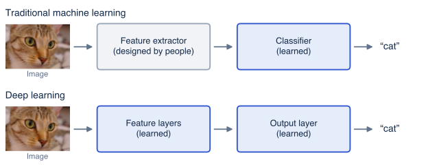
Figure 1.3 Where learning happens. Top: in traditional machine learning, people design the feature extractor (gray), and only the final classifier is learned from data (blue). Bottom: in deep learning, the layers that compute features are learned from data as well, together with the output layer.

Deep learning removes the hand-designed stage. A deep neural network is a long chain of simple computations, and all of their parameters are chosen by training (figure 1.3, bottom). The early stages end up computing features, but those features are whatever helps reduce the error on the training data, not what a person decided in advance. For images, sound and text, where good features are hard to design, this has led to large improvements in accuracy [5].

Learning the features does not mean nothing is designed. People still choose the structure of the network, the measure of error and the training data, and those choices matter a great deal. Deep learning also usually needs more data and more computation than the methods of section 3. For small tables of numbers, such as a spreadsheet of house attributes, tree-based methods remain strong competitors.

5. The plan for this course

Every supervised learning system needs answers to four questions, and each of the next articles answers one:

1. What does the model see? Article 2 explains features and how classic image features are computed.
2. What family of functions do we search? Article 3 introduces neural networks.
3. How do we measure how wrong a model is? Article 4 defines loss functions.
4. How do we find good parameters? Article 5 explains training by gradient descent.

Article 6 then asks how to tell whether the trained model is any good on data it has never seen.

Summary

A model is a function that maps inputs to outputs, and its parameters select one function from a family. Machine learning chooses those parameters from training examples instead of writing the function by hand. Traditional methods learn the final mapping but rely on hand-designed features. Deep learning learns the features too, which works especially well for images, sound and text, at the cost of more data and computation.

Notes

Reading further. Chapter 1 of Understanding Deep Learning [1] surveys supervised, unsupervised and reinforcement learning. Chapter 2 develops the straight-line model of section 2 in more detail.

Where the names come from. "Regression" means predicting a continuous number, such as a price. "Classification" means predicting a category. Both are supervised learning; they differ in the type of output, and article 4 shows that they also need different loss functions.

Extrapolation. Predicting year 10 from years 0 to 9 is extrapolation: the input lies outside the range of the training data. Models are generally less reliable there than for inputs between training examples. Article 6 returns to this.

Problems

Problem 1.1 Using the line in figure 1.2, what price does the model predict for year 12? (Answer: $1.096 + 0.0857 \times 12 \approx 2.124$.)

Problem 1.2 For each task, say whether it is regression or classification, and what the input and output are: (a) estimating a person's age from a photograph; (b) deciding whether an email is spam; (c) predicting tomorrow's maximum temperature.

Problem 1.3 A grayscale photograph has $640 \times 480$ pixels with one number per pixel. How many numbers does the model receive? How many if the photograph is in colour? (Answer: 307,200 and 921,600.)

References

• 1: Simon J.D. Prince (2023). Understanding Deep Learning. MIT Press.
• 2: Corinna Cortes and Vladimir Vapnik (1995). Support-vector networks. Machine Learning 20, 273–297.
• 3: Leo Breiman (2001). Random forests. Machine Learning 45, 5–32.
• 4: Stuart Lloyd (1982). Least squares quantization in PCM. IEEE Transactions on Information Theory 28(2), 129–137.
• 5: Yann LeCun, Yoshua Bengio and Geoffrey Hinton (2015). Deep learning. Nature 521, 436–444.