Evaluating models: will it work on new data?

Article 5 found the parameters with the lowest loss on the training data. That is not what we actually want. We want a model that makes good predictions for inputs it has never seen: next year's house price, a photograph taken tomorrow. This article shows why a low training loss does not guarantee that, how to measure performance honestly by holding data back, and which numbers are used to report performance for common tasks.

1. A perfect fit that predicts badly

We fit three models to the ten years of house prices: a constant (the same price every year), the straight line of article 1, and a polynomial of degree 9, a curve with ten parameters (figure 6.1).

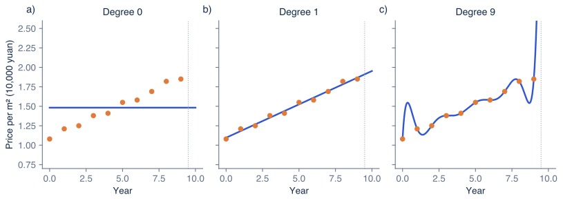
Figure 6.1 Underfitting and overfitting. Three models fitted to the house prices of years 0–9; the dotted line marks the end of the data. a) A constant: training error 0.0612; it predicts 1.48 for year 10. b) A straight line: training error 0.00063; it predicts 1.95. c) A polynomial of degree 9: training error essentially zero, because it passes through every point, but it predicts 22.47 for year 10.

Judged by training error alone, the degree-9 polynomial is the best model: it fits the ten points exactly. Yet its prediction for year 10 is more than ten times the current price. Ten parameters are enough to pass through ten points exactly, so the curve has fitted not only the trend but also the small year-to-year fluctuations, which will not repeat. This is called overfitting. The constant has the opposite problem: it is too simple to follow the trend at all, which is called underfitting. The line is flexible enough for the trend and not flexible enough for the noise.

A model's performance on new data drawn from the same source as the training data is called its generalization. Training error says nothing reliable about it, so we need another way to measure it.

2. Training, validation and test sets

The solution is to hold some data back. Before training, we split the available data into three parts:

• The training set is used to fit the parameters, as in article 5.
• The validation set is used to make choices that training itself does not make, such as the degree of the polynomial, the number of hidden units, or the learning rate. These are called hyperparameters. We train one model for each candidate setting and keep the setting with the lowest validation error.
• The test set is used once, at the very end, to estimate how well the final model will perform on new data.

Common proportions are 70/15/15 or 80/10/10, but they depend on how much data there is. Figure 6.2 shows why the validation set is needed. As the degree of a polynomial grows, the training error keeps falling, because every extra parameter gives the curve more freedom. The validation error falls at first and then rises sharply once the model starts fitting noise. Here the lowest validation error is at degree 3.

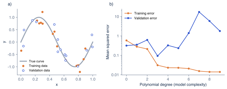
Figure 6.2 Choosing model complexity with a validation set. a) Fifteen training points (orange) and fifteen validation points (blue) drawn from the same noisy wave (gray). b) Polynomials of degree 0 to 9 fitted to the training points. The training error (orange) falls as the degree increases. The validation error (blue, on a logarithmic scale) is lowest at degree 3 and grows rapidly for higher degrees, which fit the noise in the training points.

Some projects split the data into only a training set and a test set, and use the test set to make the choices. The test error then no longer measures performance on unseen data, because the test data have influenced the model. When data are scarce, cross-validation is an alternative: the data are divided into, say, five parts; each part serves once as the validation set while the model is trained on the other four, and the five validation errors are averaged.

The split must also match how the model will be used. For the house prices, the model will predict the future, so a fair test holds back the latest years rather than a random selection. If we train on years 0–7 and test on years 8 and 9, the line predicts 1.771 and 1.855 against true values 1.82 and 1.85. The polynomial of degree 7, which fits years 0–7 exactly, predicts 8.26 and 47.85.

3. Never train on the test set

A test score is a promise: it tells readers how the model will perform on data it has never seen. That promise holds only if the test data have played no part in building the model. If they were used for training, for choosing hyperparameters, or even for deciding when to stop trying new ideas, the score is optimistically biased, sometimes by a large margin. Publishing such a score as if it were an honest estimate misleads everyone who relies on it, which is why doing so is treated as a breach of research ethics.

Test data can also leak in less obvious ways:

• Duplicates. The same or nearly the same example appears in both the training and the test set, such as two photographs of the same scene.
• Preprocessing. A step such as normalization uses statistics computed from all the data, test set included. Compute such statistics from the training set only.
• Time. A random split puts later records into training when the model is meant to predict the future.

4. Benchmarks

To compare methods fairly, a research community agrees on a benchmark: a public dataset with a fixed split into training, validation and test data, and a fixed way of measuring performance. ImageNet [2] is a classic benchmark for image classification, and COCO [3] for object detection and segmentation. Papers report their results on such benchmarks so that they can be compared directly. This is the meaning of the phrase "state of the art on benchmark X".

Benchmarks have a known weakness. When thousands of papers tune their methods on the same test set, the community as a whole can overfit to it, even if no single paper does anything wrong. Some benchmarks therefore keep their test labels secret and score submissions on a server.

5. Common evaluation metrics

The loss is chosen to make training work (article 4). For reporting, we use metrics that people can interpret, and they depend on the task.

Regression. The mean absolute error (MAE) is the average size of the errors, and the root mean squared error (RMSE) is the square root of the MSE. Both are in the units of the output. For the line trained on years 0–7 and tested on years 8 and 9, the errors are $-0.049$ and $0.005$, so the MAE is $0.027$, that is, 270 yuan per square metre.

Classification. The simplest metric is accuracy, the fraction of correct predictions. It can mislead when the categories are unbalanced: if only 2% of photographs contain cats, a model that always answers "no cat" is 98% accurate and useless. A confusion matrix gives a fuller picture. Suppose a cat detector is tested on 100 photographs, 40 of which contain cats:

	Predicted "cat"	Predicted "no cat"
Contains a cat	32 (true positives)	8 (false negatives)
No cat	6 (false positives)	54 (true negatives)

• Accuracy $= (32 + 54) / 100 = 0.86$.
• Precision asks: of the photographs the model called "cat", how many were cats? $32 / (32 + 6) = 0.842$.
• Recall asks: of the photographs that contained cats, how many did the model find? $32 / (32 + 8) = 0.80$.
• The F1 score combines the two: $2 \times 0.842 \times 0.80 / (0.842 + 0.80) = 0.821$.

Precision matters when false alarms are costly, such as a spam filter that hides real email. Recall matters when misses are costly, such as a medical screening test.

Detection. A predicted box counts as correct only if it overlaps the true box enough. The overlap is measured by the intersection over union (IoU): the area covered by both boxes divided by the area covered by either. Two $50 \times 50$ boxes offset by 20 pixels horizontally and 10 vertically share an area of $30 \times 40 = 1200$, and together cover $2500 + 2500 - 1200 = 3800$, so their IoU is $1200 / 3800 = 0.32$. A common rule requires an IoU of at least 0.5, so this prediction would count as a miss. Detection benchmarks summarise precision and recall over all confidence levels into the mean average precision (mAP), often averaged over several IoU thresholds.

Segmentation. The IoU is computed between the predicted and true pixel regions of each category and averaged over categories, giving the mean IoU. The closely related Dice coefficient is common in medical imaging.

Text. Language models are often evaluated by perplexity, which measures how probable the model finds held-out text. Machine translation and summarisation have traditionally been measured by counting word sequences shared with reference texts, as BLEU [4] and ROUGE [5] do.

Task	Common metrics
Regression	MAE, RMSE
Classification	Accuracy, precision, recall, F1
Object detection	IoU, mAP
Segmentation	Mean IoU, Dice
Text generation	Perplexity, BLEU, ROUGE

Summary

A low training loss does not guarantee good predictions on new data: a model that is too flexible fits the noise in its training data and generalizes badly. To measure performance honestly, we split the data into a training set for fitting the parameters, a validation set for choosing hyperparameters, and a test set used once at the end. Test data must never influence the model. Benchmarks fix datasets, splits and metrics so that methods can be compared. Metrics depend on the task: MAE and RMSE for regression, accuracy, precision, recall and F1 for classification, IoU and mAP for detection.

This completes the beginner part of the course. With these six ideas, a model, its features, a network, a loss, training and evaluation, it is possible to read most introductory deep learning code and papers. The next part will build on them.

Notes

Bias and variance. The two failure modes of figure 6.1 are often described as bias, error from a model too simple for the true relationship, and variance, error from a model so flexible that it depends on the particular noise in the training data. Chapter 8 of Understanding Deep Learning [1] analyses them and the surprising behaviour of very large networks, called double descent, where test error can fall again as models grow far beyond the size needed to fit the training data.

Regularization. Besides choosing a simpler model, overfitting can be reduced by penalizing large parameter values, by stopping training early when the validation error starts to rise, or by collecting more data. Chapter 9 of Understanding Deep Learning [1] covers these methods.

Metrics follow decisions. No metric is right for every use. A model for screening rare diseases and a model for recommending films need different trade-offs between precision and recall, and the choice should come from the cost of each kind of mistake.

Problems

Problem 6.1 Using the confusion matrix in section 5, suppose the detector is changed so that it now predicts "cat" for 50 photographs, 38 of which contain cats. Compute the new precision and recall. (Answer: precision $38/50 = 0.76$, recall $38/40 = 0.95$.)

Problem 6.2 Two boxes of size $40 \times 40$ overlap in a $20 \times 40$ region. What is their IoU? (Answer: $800 / (1600 + 1600 - 800) = 1/3$.)

Problem 6.3 A student tries 200 different settings of hyperparameters and reports the best test accuracy among them. Explain why this number is likely to overestimate the accuracy on new data.

References

• 1: Simon J.D. Prince (2023). Understanding Deep Learning. MIT Press.
• 2: Jia Deng, Wei Dong, Richard Socher, Li-Jia Li, Kai Li and Li Fei-Fei (2009). ImageNet: a large-scale hierarchical image database. Conference on Computer Vision and Pattern Recognition.
• 3: Tsung-Yi Lin and colleagues (2014). Microsoft COCO: common objects in context. European Conference on Computer Vision.
• 4: Kishore Papineni, Salim Roukos, Todd Ward and Wei-Jing Zhu (2002). BLEU: a method for automatic evaluation of machine translation. Annual Meeting of the Association for Computational Linguistics.
• 5: Chin-Yew Lin (2004). ROUGE: a package for automatic evaluation of summaries. Text Summarization Branches Out.