Deep networks: why depth helps

Article 3 built a shallow network, one hidden layer of ReLU units, and showed that it describes piecewise linear functions: each hidden unit adds one joint, and with enough units the network can approximate any continuous function. It ended by claiming that stacking layers creates joints "far more economically" and that this is why modern networks are deep. This article makes that claim precise. We compose two small networks by hand and count the pieces, show that the composition is a special case of a network with two hidden layers, write down the general deep network in matrix form, and then ask what depth does and does not buy: in what can be represented, in what can be trained, and in what generalizes.

Part 2 assumes the material of part 1: models, losses, gradient descent, backpropagation in outline, and overfitting. It also assumes matrix products, transposes and partial derivatives. New notation is collected on the notation page.

1. Composing two networks

We start with two shallow networks of exactly the kind in article 3: one input, three ReLU hidden units, one output. We defer the general deep network until section 3. The first network maps $x$ to $y$:

$$y = f(x) = \phi_0 + \sum_{d=1}^{3} \phi_d \,\mathrm{ReLU}(\theta_{d0} + \theta_{d1} x) \tag{7.1}$$

The second network has the same form but its own parameters, which we call $\psi$ ("psi") for the hidden units and $\phi'$ for the output. It maps $y$ to a new output $y'$:

$$y' = g(y) = \phi'_0 + \sum_{d=1}^{3} \phi'_d \,\mathrm{ReLU}(\psi_{d0} + \psi_{d1} y) \tag{7.2}$$

Composing the networks means feeding the output of the first into the second: $y' = g(f(x))$. Nothing about either network changes. We only connect them in series.

We choose parameters that make the effect easy to see. Both networks place their three hidden units at the same positions: $(\theta_{d0}, \theta_{d1}) = (0, 1), (-1, 1), (-2, 1)$ for $d = 1, 2, 3$, and the same values for $(\psi_{d0}, \psi_{d1})$. The units therefore switch on at inputs 0, 1 and 2. The output weights differ:

	Output offset	Output weights
Network 1, $f$	$\phi_0 = 0$	$(\phi_1, \phi_2, \phi_3) = (3, -6, 6)$
Network 2, $g$	$\phi'_0 = 0.5$	$(\phi'_1, \phi'_2, \phi'_3) = (1, -2, 1.5)$

We look only at inputs between 0 and 3. On that range, network 1 is a zigzag (figure 7.1a). Between 0 and 1 only unit 1 is on, so $f(x) = 3x$, which rises from 0 to 3. Between 1 and 2 unit 2 is on as well, the slope becomes $3 - 6 = -3$, and $f$ falls from 3 back to 0. Between 2 and 3 all three units are on, the slope is $3 - 6 + 6 = 3$, and $f$ rises from 0 to 3 again. Network 1 maps each of the three intervals $[0, 1]$, $[1, 2]$ and $[2, 3]$ onto the whole range $[0, 3]$, the middle one in reverse.

Network 2 is a different three-piece function on the same range (figure 7.1b): slope 1 between 0 and 1, slope $1 - 2 = -1$ between 1 and 2, and slope $1 - 2 + 1.5 = 0.5$ between 2 and 3.

Take $x = 1.5$. In network 1, the three pre-activations are $1.5$, $0.5$ and $-0.5$, so the hidden units are $1.5$, $0.5$ and $0$, and $y = 3 \times 1.5 - 6 \times 0.5 + 6 \times 0 = 1.5$. In network 2 the input is $y = 1.5$, which happens to give the same hidden values, and $y' = 0.5 + 1 \times 1.5 - 2 \times 0.5 + 1.5 \times 0 = 1.0$.

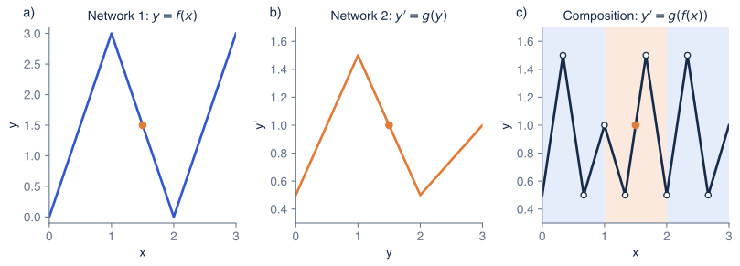
Figure 7.1 Composing two shallow networks. a) Network 1 (equation 7.1) with the parameters of section 1 is a zigzag with three pieces on $[0, 3]$: it maps each third of the input range onto the whole range $[0, 3]$. b) Network 2 (equation 7.2) has three pieces with slopes 1, $-1$ and $0.5$. c) The composition $g(f(x))$ has nine pieces. In each shaded third of the input range, network 2's whole shape appears once, compressed by a factor of 3; in the middle third it is mirrored, because $f$ runs backwards there. The orange dots follow the worked example $x = 1.5 \to y = 1.5 \to y' = 1.0$.

Figure 7.1c shows the result. As $x$ moves from 0 to 1, $y = f(x)$ sweeps the whole range $[0, 3]$, so $y'$ traces the whole of network 2's function. As $x$ moves from 1 to 2, $y$ sweeps the range again backwards, and $y'$ traces network 2's function in mirror image. From 2 to 3 it traces it once more. Each copy keeps network 2's three pieces, so the composition has $3 \times 3 = 9$ linear pieces, joined at $x = 1/3, 2/3, 1, 4/3, \ldots, 8/3$.

The slopes confirm this. By the chain rule, the slope of $g(f(x))$ is the slope of $g$ at $y = f(x)$ times the slope of $f$ at $x$. On the first ninth, both are increasing: $1 \times 3 = 3$. On the second ninth, $g$ has slope $-1$ while $f$ still rises: $-1 \times 3 = -3$. The nine slopes are $3, -3, 1.5, -1.5, 3, -3, 3, -3, 1.5$, and each differs from its neighbour, so all eight joints are genuine.

This is the central picture of the article. Network 1 folds the input range onto itself, three layers of paper stacked on top of each other. Network 2 then draws one function on the folded paper. When the paper is unfolded, the drawing appears on every layer. Two networks with three hidden units each produce nine pieces; a single shallow network with six hidden units can produce at most seven, because each unit adds at most one joint.

2. A composition is a deep network

The composition of section 1 is a network with two hidden layers in disguise. To see this, we substitute the output of network 1 into the hidden units of network 2. Unit $d$ of network 2 computes:

$$\begin{aligned} h'_d &= \mathrm{ReLU}\big(\psi_{d0} + \psi_{d1}\, y\big) \\ &= \mathrm{ReLU}\Big(\psi_{d0} + \psi_{d1}\big(\phi_0 + \textstyle\sum_{j=1}^{3} \phi_j h_j\big)\Big) \\ &= \mathrm{ReLU}\Big(\underbrace{(\psi_{d0} + \psi_{d1}\phi_0)}_{\text{offset}} + \textstyle\sum_{j=1}^{3} \underbrace{\psi_{d1}\phi_j}_{\text{weight}}\, h_j\Big) \end{aligned} \tag{7.3}$$

where $h_1, h_2, h_3$ are the hidden units of network 1. The first line is equation 7.2's hidden unit. The second substitutes equation 7.1 for $y$. The third collects terms: everything that does not multiply an $h_j$ is an offset, and the coefficient of each $h_j$ is a weight.

In words: the second set of hidden units takes the first set as its inputs, through its own offsets and weights. That is exactly a second hidden layer. The output $y'$ is then a weighted sum of $h'_1, h'_2, h'_3$, as in any network.

For our numbers, the weight from first-layer unit $j$ to second-layer unit $d$ is $\psi_{d1}\phi_j$. Since every $\psi_{d1} = 1$ and $\phi = (3, -6, 6)$, all three second-layer units receive the same weights, and the offsets are $\psi_{d0} + \psi_{d1}\phi_0 = 0, -1, -2$:

$$\boldsymbol{\Omega}_1 = \begin{bmatrix} 3 & -6 & 6 \\ 3 & -6 & 6 \\ 3 & -6 & 6 \end{bmatrix}, \qquad \boldsymbol{\beta}_1 = \begin{bmatrix} 0 \\ -1 \\ -2 \end{bmatrix}$$

The matrix has a special structure: each row is a multiple of the same vector $\boldsymbol{\phi}$, so it has rank one. This is the restriction that composing two separate networks imposes. A general network with two hidden layers lets all nine entries of $\boldsymbol{\Omega}_1$ be chosen freely. It can therefore represent every composition of two shallow networks with three units each, and many functions besides. In the general network the second layer has 9 free weights and 3 offsets, 12 numbers; the composition derives all 12 from only 10 (network 1's four output parameters and network 2's six hidden-unit parameters). The composition therefore has 20 parameters, and the general network with layers of sizes 1, 3, 3 and 1 has 22 (section 3 counts them).

This explains what the second layer does in general. Each first-layer unit produces a piecewise linear function of the input. Each second-layer unit takes a weighted combination of those functions, which is again piecewise linear, and clips it at zero with the ReLU. Clipping a function that crosses zero many times adds a new joint at every crossing. In section 1 the combination was the zigzag $f$, and the units of the second layer cut it at the heights 0, 1 and 2.

3. The general deep network

A network with $K$ hidden layers computes a sequence of vectors $\mathbf{h}_1, \ldots, \mathbf{h}_K$. Each layer applies an affine map to the previous vector and then the activation function:

$$\begin{aligned} \mathbf{h}_1 &= a\big(\boldsymbol{\beta}_0 + \boldsymbol{\Omega}_0 \mathbf{x}\big) \\ \mathbf{h}_{k+1} &= a\big(\boldsymbol{\beta}_k + \boldsymbol{\Omega}_k \mathbf{h}_k\big), \qquad k = 1, \ldots, K - 1 \\ \mathbf{y} &= \boldsymbol{\beta}_K + \boldsymbol{\Omega}_K \mathbf{h}_K \end{aligned} \tag{7.4}$$

We can break this down into three parts. The first line maps the input $\mathbf{x}$, with $D_i$ elements, to the first hidden layer $\mathbf{h}_1$, with $D_1$ elements; this is the hidden layer of article 3 in matrix form. The second line repeats the same operation for each later layer, using the previous layer's values as inputs. The last line is linear, with no activation, so that the output can take any value; for classification the softmax of article 4 is applied afterwards, as part of the loss. In words: a deep network alternates affine maps and elementwise activations, and ends with an affine map.

To complete the description, we state the shapes. Layer $k$ has $D_k$ hidden units, and we write $D_0 = D_i$ for the input size and $D_{K+1} = D_o$ for the output size. Then:

• $\boldsymbol{\Omega}_k \in \mathbb{R}^{D_{k+1} \times D_k}$ is the weight matrix that maps layer $k$ to layer $k+1$. Its entry in row $d$ and column $j$ is the weight from unit $j$ of layer $k$ to unit $d$ of layer $k+1$.
• $\boldsymbol{\beta}_k \in \mathbb{R}^{D_{k+1}}$ is the bias vector added in layer $k+1$.
• $a(\cdot)$ is applied to each element separately. We use ReLU unless stated otherwise.

The notation connects directly to article 3. A shallow network is the case $K = 1$: $\boldsymbol{\beta}_0$ and $\boldsymbol{\Omega}_0$ hold the hidden units' offsets $\theta_{d0}$ and weights $\theta_{dj}$, and $\boldsymbol{\beta}_1$ and $\boldsymbol{\Omega}_1$ hold the output offset $\phi_0$ and weights $\phi_d$. From here on we index the layers rather than giving each its own Greek letter.

Each layer has $D_{k+1} D_k$ weights and $D_{k+1}$ biases, so the network has

$$P = \sum_{k=0}^{K} D_{k+1}\,(D_k + 1) \tag{7.5}$$

parameters. For the network of section 2, with sizes $(1, 3, 3, 1)$, this is $3 \times 2 + 3 \times 4 + 1 \times 4 = 22$. A classifier for $28 \times 28$ grayscale digit images with two hidden layers of 256 units and 10 outputs, sizes $(784, 256, 256, 10)$, has $256 \times 785 + 256 \times 257 + 10 \times 257 = 269{,}322$ parameters. Most of them sit in the first layer, because the input is large.

The numbers $K$ and $D_1, \ldots, D_K$ are fixed before training and are not changed by gradient descent. They are hyperparameters, chosen with a validation set as in article 6. $K$ is the network's depth and $D_k$ is the width of layer $k$. Most fully connected networks use the same width for every hidden layer, and the choice is then two numbers.

4. Counting linear regions

With ReLU activations, every network of the form of equation 7.4 computes a piecewise linear function: the input space is divided into regions, and inside each region the output is an affine function of the input. Counting the regions is a way to measure how complicated a function the network can make. This section counts them for shallow and deep networks.

Shallow networks

The regions come from the hidden units switching on and off. For a fixed input, each ReLU unit is either active (positive pre-activation, passes its value) or inactive (outputs zero). If we fix which units are active, every ReLU becomes either the identity or zero, and the network becomes an affine function of the input. A region is therefore a set of inputs that share the same activation pattern, and a joint is where some unit's pre-activation crosses zero.

With one input and $D$ hidden units, each unit's pre-activation $\theta_{d0} + \theta_{d1}x$ crosses zero at one point, so the network has at most $D$ joints and $D + 1$ pieces. With $D_i$ inputs, the zero set of unit $d$, $\{\mathbf{x} : \theta_{d0} + \boldsymbol{\theta}_d^\top \mathbf{x} = 0\}$, is a hyperplane: a line when $D_i = 2$, a plane when $D_i = 3$. $D$ hyperplanes in general position divide $D_i$-dimensional space into

$$N_{\text{shallow}} = \sum_{j=0}^{D_i} \binom{D}{j} \tag{7.6}$$

regions, a classical result of geometry [5]. Here $\binom{D}{j}$ is the number of ways to choose $j$ of the $D$ hyperplanes. For one input the sum is $1 + D$, as before. For two inputs and three hidden units it is $1 + 3 + 3 = 7$: three lines in general position cut the plane into seven pieces. When $D \le D_i$ the sum equals $2^D$, because every activation pattern is possible. When $D$ is much larger than $D_i$, it grows like $D^{D_i}$: polynomially in the width.

Deep networks

Section 1 suggests that depth multiplies the count. Network 1 folds $[0, 3]$ onto itself three times. If we feed its output into another copy of network 1, each of the three folds is folded again, giving nine pieces. A third copy gives 27 (figure 7.2). As in section 2, $K$ copies in series form a network with $K$ hidden layers of width 3, sizes $(1, 3, \ldots, 3, 1)$. On $[0, 3]$ this network has exactly

$$N_{\text{deep}} = 3^K \tag{7.7}$$

linear pieces, and by equation 7.5 it has $6 + 12(K - 1) + 4 = 12K - 2$ parameters.

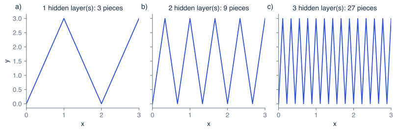
Figure 7.2 Repeated folding. The network of figure 7.1a composed with itself. a) One hidden layer of three units: 3 pieces on $[0, 3]$. b) Two hidden layers: 9 pieces. c) Three hidden layers: 27 pieces. Each extra layer of three units multiplies the number of pieces by three and adds 12 parameters.

A shallow network with the same parameter count does much worse. With one input, $D$ hidden units have $3D + 1$ parameters, so $12K - 2$ parameters buy $D = 4K - 1$ units and at most $4K$ pieces:

Hidden layers $K$	Parameters	Deep network: pieces	Shallow network, same parameters: at most
1	10	3	4
2	22	9	8
3	34	27	12
4	46	81	16
5	58	243	20

The deep count grows exponentially in the number of parameters; the shallow count grows linearly. The construction generalizes: Montúfar and colleagues [3] built deep networks with many inputs whose number of regions grows exponentially in depth, while equation 7.6 shows that the shallow count grows only polynomially in width. These are statements about the maximum: they say that some choice of parameters achieves the count.

What networks actually compute

The maximum is not what a typical network has. Figure 7.3 adds a third curve: networks of width 8 with depths 1 to 8, with weights drawn at random as at the start of training (He initialization, article 5) and small random biases. We count their pieces on the input range $[-3, 3]$ and average over 30 draws. A depth-1 network has 8.8 pieces on average and a depth-8 network, with 64 hidden units, has 57.3. The count grows roughly in proportion to the number of hidden units, and stays close to the shallow maximum $D + 1$, nowhere near $3^K$.

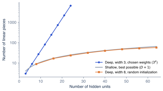
Figure 7.3 Maximum and typical numbers of linear pieces (one input). Blue: the folding networks of figure 7.2, width 3 with chosen weights, reach $3^K$ pieces with $3K$ hidden units. Gray: the most a shallow network with $D$ units can make, $D + 1$. Orange: deep networks of width 8 and depth 1 to 8 with randomly initialized weights, average count on $[-3, 3]$ over 30 draws. Note the logarithmic vertical axis. Random deep networks have about one piece per hidden unit, far below the maximum.

This matches a careful study by Hanin and Rolnick [6]. They proved that, for networks initialized in the usual way, the average number of regions that a line through input space crosses is governed by the total number of hidden units and grows roughly in proportion to it, not exponentially with depth. They also found empirically that the count stays of the same order during training. The folding construction needs weights tuned so that every fold lands exactly on top of the others. Random weights almost never line up like that.

5. What depth does and does not buy

We now have three facts that pull in different directions. Shallow networks are already universal approximators (article 3), so depth adds nothing to what can be represented in the limit of many units. Deep networks can make exponentially more pieces than shallow ones with the same parameters. And typical deep networks do not come close to that maximum. This section sorts out what is known, keeping representability, trainability and generalization apart.

Depth makes some functions much cheaper to represent. This is a theorem, not an observation. Telgarsky [4] proved that for every positive integer $k$ there is a function computed by a ReLU network with on the order of $k^3$ layers and a constant number of units per layer, which no network with on the order of $k$ layers can approximate unless it has at least on the order of $2^k$ units. The function is a sawtooth, the same mechanism as figure 7.2. Eldan and Shamir [7] showed a related separation between two and three hidden layers for a function of many inputs. These results say that depth can be exponentially more efficient. They do not say that the functions we need in practice, such as a map from images to labels, are of this kind. That question is open.

Depth does not by itself make training easier. The function computed by a deep network is a composition of many layers, so its derivatives are products of many factors (article 8 derives them). Products of many factors tend to become very large or very small, and the loss surfaces of deep networks without special design are hard to optimize. He and colleagues observed that a plain network with 56 layers had higher training error than one with 20 layers on the same task [8]. That is not overfitting, which would show up only on held-out data; the deeper network failed to fit the training set. Article 11 explains the residual connections and normalization that fixed this, and they are why networks with hundreds of layers are trainable today.

Depth tends to help generalization in practice, for reasons that are not fully understood. On images, speech and text, deeper networks have consistently reached lower test error than shallow networks of similar size, once the training problems above were solved. One experiment separates representation from learning. Ba and Caruana [9] trained shallow networks to imitate the outputs of a deep network, rather than the original labels, and the shallow networks came close to the deep network's accuracy, while shallow networks trained on the labels directly did not. The shallow networks could represent a good function; training on the labels did not find it. So part of the benefit of depth is in how well training and generalization work, not only in what can be represented.

In short: depth is useful because it can represent some functions far more cheaply, and because, with the right architecture, deep networks train to solutions that generalize well. The first is a theorem about specific functions. The second is an empirical finding with only partial theory behind it.

6. Computing with batches: shapes, operations and memory

Equation 7.4 processes one input. In training and in most deployments, a network processes a batch of $B$ inputs at once (article 5), and the computation becomes a sequence of matrix products. We collect the inputs as the columns of a matrix $\mathbf{X} \in \mathbb{R}^{D_i \times B}$. The first layer computes:

$$\mathbf{H}_1 = a\big(\boldsymbol{\beta}_0 \mathbf{1}^\top + \boldsymbol{\Omega}_0 \mathbf{X}\big) \tag{7.8}$$

where $\mathbf{1}$ is a vector of $B$ ones, so that $\boldsymbol{\beta}_0 \mathbf{1}^\top$ is a $D_1 \times B$ matrix with the bias vector in every column. The product $\boldsymbol{\Omega}_0 \mathbf{X}$ has shape $(D_1 \times D_i)(D_i \times B) = D_1 \times B$: column $b$ is the pre-activation for example $b$. In words: the same weights are applied to every example, and the batch dimension just comes along. Later layers work the same way, giving $\mathbf{H}_k \in \mathbb{R}^{D_k \times B}$.

Most deep learning libraries store a batch the other way round, one example per row, and compute $\mathbf{X}\boldsymbol{\Omega}^\top$. That is the same computation transposed. We keep one example per column, matching the vectors of equation 7.4.

Three quantities describe the cost, and they should not be confused:

• Parameters are the numbers that training changes. They do not depend on $B$. The $(784, 256, 256, 10)$ classifier has 269,322; stored as 32-bit floating-point numbers they take about 1.08 MB.
• Operations. A layer multiplies a $D_{k+1} \times D_k$ matrix by a $D_k \times B$ matrix, which takes $D_{k+1} D_k B$ multiply-adds. For the classifier this is $784 \times 256 + 256 \times 256 + 256 \times 10 = 268{,}800$ multiply-adds per example, or about 68.8 million for a batch of 256. The bias additions and activations are negligible next to the products. Article 8 shows that the backward pass costs about twice as much again.
• Activations are the intermediate values $\mathbf{H}_k$. Their size is $B \sum_k D_k$, and training must keep them until the backward pass has used them (article 8). For large models and batches, activations, not parameters, often dominate memory.

Fully connected layers make every unit depend on every unit of the previous layer, and that is costly when inputs are large. A $224 \times 224$ color image has 150,528 input values, so one fully connected layer of 1,000 units would need about 150 million weights. Convolutional networks (article 10) and transformers (article 12) are deep networks whose layers share weights to avoid this.

7. Terminology

With the general network in hand, we can name its parts and settle some ambiguous usage.

• A network built from equation 7.4 is a deep fully connected network, also called a multilayer perceptron or MLP. "Deep" has no exact threshold; in practice it means more than one hidden layer.
• The depth $K$ is the number of hidden layers, and the width of a layer is its number of hidden units. Papers count layers inconsistently: some count weight matrices, so that our $(784, 256, 256, 10)$ classifier is a "three-layer network", and others count hidden layers, making it a "two-hidden-layer network". Say which one you mean.
• The values before the activation, $\boldsymbol{\beta}_k + \boldsymbol{\Omega}_k \mathbf{h}_k$, are pre-activations; the values after are activations, as in article 3.
• The activation pattern of an input is the set of active ReLU units. Each pattern that occurs defines one linear region, inside which the network is an affine function.
• The capacity of a network is an informal word for how complicated a function it can represent. The number of linear regions is one way to make it concrete; the parameter count is another, cruder one.
• The choice of depth, widths, activation function and connection pattern is the network's architecture. Its numbers are hyperparameters, set before training, as opposed to the parameters that training adjusts.

Summary

Composing two shallow networks feeds the output of one into the other. When the first network folds its input range onto itself, the second network's function appears once on every fold, so the pieces multiply: two networks with three units each make nine pieces, where a single network with six units makes at most seven. Substituting one network into the other shows that a composition is a network with two hidden layers whose second weight matrix has rank one; the general deep network of equation 7.4 frees that matrix and repeats the pattern for $K$ layers. Repeated folding gives $3^K$ pieces with $12K - 2$ parameters, against at most $4K$ for a shallow network, and theorems confirm that depth can be exponentially more efficient for some functions. These are maximums: randomly initialized networks have roughly one piece per hidden unit. Depth also makes training harder, and its practical benefit comes from deep architectures that train well and generalize well, which the next articles develop. Article 8 starts with the derivatives that training needs.

Notes

The general lower bound. For $D_i$ inputs and $K$ hidden layers of width $D \ge D_i$, Montúfar and colleagues [3] showed that the maximum number of linear regions is at least $\lfloor D / D_i \rfloor^{D_i (K-1)} \sum_{j=0}^{D_i} \binom{D}{j}$: exponential in depth, polynomial in width. Later work tightened both lower and upper bounds. With $D_i = 1$ and $D = 3$ the bound is $4 \times 3^{K-1}$, slightly more than our $3^K$ because it counts the whole real line, not only $[0, 3]$.

Width matters too. Depth is not free of conditions. A ReLU network whose layers are all narrower than or equal to its number of inputs cannot be a universal approximator, however deep it is: the image of each layer has too few dimensions to separate some inputs. Universal approximation by deep narrow ReLU networks needs a width of at least $D_i + 1$ [10]; the exact threshold depends on the number of outputs and on how the approximation error is measured.

Linear networks. Without activation functions, equation 7.4 collapses to $\mathbf{y} = \boldsymbol{\Omega}\mathbf{x} + \boldsymbol{\beta}$ with $\boldsymbol{\Omega} = \boldsymbol{\Omega}_K \cdots \boldsymbol{\Omega}_0$ (article 3, section 5). The product can be no higher in rank than the narrowest layer, so a narrow hidden layer limits a linear network. Deep linear networks represent nothing new, but their training dynamics are nonlinear and are a standard model for studying how depth affects optimization.

Other activation functions. With smooth activations such as GELU or tanh, the network is no longer piecewise linear and "counting regions" no longer applies, but the composition picture still holds: each layer bends and folds the representation of the previous layer.

Reading further. Chapter 4 of Understanding Deep Learning [1] covers composing networks, the general deep network and the depth-efficiency results, with interactive figures. Goodfellow, Bengio and Courville [2], section 6.4, discuss architecture design and depth.

Problems

Problem 7.1 Using the parameters of section 1, compute $f(0.2)$ and $g(f(0.2))$. (Answer: $f(0.2) = 0.6$, and $g(0.6) = 0.5 + 0.6 = 1.1$.)

Problem 7.2 How many parameters does a fully connected network with sizes $(10, 20, 20, 2)$ have? (Answer: $20 \times 11 + 20 \times 21 + 2 \times 21 = 682$.)

Problem 7.3 Network 1 composed with itself, $f(f(x))$, is a network with two hidden layers. Write down its $\boldsymbol{\beta}_1$ and $\boldsymbol{\Omega}_1$. (Answer: the same as in section 2, $\boldsymbol{\beta}_1 = (0, -1, -2)^\top$ and every row of $\boldsymbol{\Omega}_1$ equal to $(3, -6, 6)$, because network 2's hidden units have the same parameters as network 1's.)

Problem 7.4 Into how many regions can a shallow network with two inputs and four hidden units divide the plane? How many if it had four inputs? (Answer: $1 + 4 + 6 = 11$ for two inputs; $1 + 4 + 6 + 4 + 1 = 16 = 2^4$ for four.)

Problem 7.5 The folding network with four hidden layers of width 3 has how many pieces on $[0, 3]$ and how many parameters? What is the most a shallow network with the same number of parameters can make? (Answer: 81 pieces and 46 parameters; a shallow network with 46 parameters has 15 units and at most 16 pieces.)

Problem 7.6 Show that a network with two hidden layers and no activation functions, $\mathbf{y} = \boldsymbol{\beta}_2 + \boldsymbol{\Omega}_2(\boldsymbol{\beta}_1 + \boldsymbol{\Omega}_1(\boldsymbol{\beta}_0 + \boldsymbol{\Omega}_0\mathbf{x}))$, is an affine function of $\mathbf{x}$, and give its weight matrix and bias. If the sizes are $(100, 10, 50, 100)$, what is the largest possible rank of the weight matrix? (Answer: weight $\boldsymbol{\Omega}_2\boldsymbol{\Omega}_1\boldsymbol{\Omega}_0$ and bias $\boldsymbol{\beta}_2 + \boldsymbol{\Omega}_2\boldsymbol{\beta}_1 + \boldsymbol{\Omega}_2\boldsymbol{\Omega}_1\boldsymbol{\beta}_0$; the rank is at most 10, the width of the narrowest layer.)

Problem 7.7 How many multiply-adds does one example need in a fully connected network of sizes $(3072, 1024, 1024, 10)$, ignoring biases and activations? (Answer: $3{,}145{,}728 + 1{,}048{,}576 + 10{,}240 = 4{,}204{,}544$.)

References

• 1: Simon J.D. Prince (2023). Understanding Deep Learning. MIT Press.
• 2: Ian Goodfellow, Yoshua Bengio and Aaron Courville (2016). Deep Learning. MIT Press.
• 3: Guido Montúfar, Razvan Pascanu, Kyunghyun Cho and Yoshua Bengio (2014). On the number of linear regions of deep neural networks. Advances in Neural Information Processing Systems 27.
• 4: Matus Telgarsky (2016). Benefits of depth in neural networks. Conference on Learning Theory.
• 5: Thomas Zaslavsky (1975). Facing up to arrangements: face-count formulas for partitions of space by hyperplanes. Memoirs of the American Mathematical Society 154.
• 6: Boris Hanin and David Rolnick (2019). Complexity of linear regions in deep networks. International Conference on Machine Learning.
• 7: Ronen Eldan and Ohad Shamir (2016). The power of depth for feedforward neural networks. Conference on Learning Theory.
• 8: Kaiming He, Xiangyu Zhang, Shaoqing Ren and Jian Sun (2016). Deep residual learning for image recognition. IEEE Conference on Computer Vision and Pattern Recognition.
• 9: Lei Jimmy Ba and Rich Caruana (2014). Do deep nets really need to be deep? Advances in Neural Information Processing Systems 27.
• 10: Boris Hanin and Mark Sellke (2017). Approximating continuous functions by ReLU nets of minimal width. arXiv:1710.11278.