Backpropagation: every gradient in one backward pass

Gradient descent needs the derivative of the loss with respect to every parameter (article 5). Article 5 computed these derivatives by hand for a network with one hidden unit, and article 7 introduced deep networks whose parameters number in the hundreds of thousands. This article derives the algorithm that computes all of these derivatives at once, backpropagation, in full. We first run it on a chain of scalar functions with actual numbers, then state the general rule for any computation, then derive the matrix form for a deep network and work through an example. We then count its cost in operations and memory, show how the backward pass starts from the loss, place it within automatic differentiation, and finally use the backward equations to explain why the scale of the initial weights decides whether a deep network trains at all.

1. Why we need an algorithm

The simplest way to estimate a derivative is to nudge a parameter and measure the change in the loss. The central difference

$$\frac{\partial \ell}{\partial \phi} \approx \frac{\ell(\phi + \epsilon) - \ell(\phi - \epsilon)}{2\epsilon} \tag{8.1}$$

needs two evaluations of the loss for each parameter, each a full forward pass through the network. For the $(784, 256, 256, 10)$ classifier of article 7, with 269,322 parameters, one gradient would cost 538,644 forward passes. Gradient descent takes thousands of steps, so this is hopeless.

Two observations point to a better method. First, a weight multiplies an activation, so its effect on the loss is proportional to that activation: if the activation is zero, changing the weight does nothing, and if it is large, a small change in the weight has a large effect. Second, a parameter in an early layer affects the loss only through all the layers after it. Every early parameter shares the same downstream path, so the derivatives along that path can be computed once and reused. Backpropagation exploits both: it computes the derivatives with respect to the intermediate values, starting at the loss and working backwards, and then reads off each parameter's derivative from the intermediate value it feeds and the activation it multiplies.

2. A chain of functions

We start with a model that is a chain of scalar operations, the smallest case that has all of backpropagation's steps. We defer the network version until section 4. With one input $x$, the model computes:

$$\begin{aligned} f_0 &= \beta_0 + \omega_0 x, & h_1 &= \sin(f_0), \\ f_1 &= \beta_1 + \omega_1 h_1, & h_2 &= \exp(f_1), \\ f_2 &= \beta_2 + \omega_2 h_2, & h_3 &= \cos(f_2), \\ f_3 &= \beta_3 + \omega_3 h_3, & \ell &= (f_3 - y)^2 \end{aligned} \tag{8.2}$$

It has the structure of a deep network with one unit per layer. Each $f_k$ is an affine function with a bias $\beta_k$ and a weight $\omega_k$ ("omega"), and each $h_{k+1}$ applies a nonlinear function to it. We use three different nonlinear functions instead of ReLU so that every step of the derivation looks different. The last line is the squared error for one training example $(x, y)$. The model has eight parameters.

We take $x = 0.6$, $y = 0.4$ and the parameter values $\beta_0 = 0.1$, $\omega_0 = 1.2$, $\beta_1 = -0.3$, $\omega_1 = 0.8$, $\beta_2 = 0.2$, $\omega_2 = 0.5$, $\beta_3 = 0.1$, $\omega_3 = 1.5$.

The forward pass evaluates equation 8.2 from top to bottom and stores every intermediate value: $f_0 = 0.1 + 1.2 \times 0.6 = 0.82$, $h_1 = \sin 0.82 = 0.7311$, $f_1 = -0.3 + 0.8 \times 0.7311 = 0.2849$, $h_2 = e^{0.2849} = 1.3297$, $f_2 = 0.8648$, $h_3 = \cos 0.8648 = 0.6488$, $f_3 = 1.0732$ and finally $\ell = (1.0732 - 0.4)^2 = 0.4531$.

The backward pass computes the derivative of the loss with respect to each intermediate value, in the opposite order. We start at the end:

$$\frac{\partial \ell}{\partial f_3} = 2(f_3 - y) = 1.3463$$

The value $h_3$ affects the loss only through $f_3 = \beta_3 + \omega_3 h_3$, which grows by $\omega_3$ for every unit of $h_3$. By the chain rule:

$$\frac{\partial \ell}{\partial h_3} = \frac{\partial f_3}{\partial h_3}\,\frac{\partial \ell}{\partial f_3} = \omega_3 \times 1.3463 = 2.0195$$

Next, $f_2$ affects the loss only through $h_3 = \cos f_2$, whose derivative is $-\sin f_2$:

$$\frac{\partial \ell}{\partial f_2} = \frac{\partial h_3}{\partial f_2}\,\frac{\partial \ell}{\partial h_3} = -\sin(0.8648) \times 2.0195 = -1.5368$$

The pattern repeats down the chain. Each step multiplies the derivative computed in the previous step by one local derivative, the derivative of a single operation with respect to its input:

$$\frac{\partial \ell}{\partial h_k} = \omega_k \frac{\partial \ell}{\partial f_k}, \qquad \frac{\partial \ell}{\partial f_{k-1}} = a_k'(f_{k-1})\,\frac{\partial \ell}{\partial h_k} \tag{8.3}$$

where $a_k$ is the nonlinear function of step $k$ (sin, exp or cos here). In words: to move back past an affine step, multiply by its weight; to move back past a nonlinear step, multiply by the slope of the function at the value it received in the forward pass. The second rule is why the forward pass stored the $f_k$. Continuing gives $\partial\ell/\partial h_2 = -0.7684$, $\partial\ell/\partial f_1 = e^{0.2849} \times (-0.7684) = -1.0217$, $\partial\ell/\partial h_1 = -0.8174$ and $\partial\ell/\partial f_0 = \cos(0.82) \times (-0.8174) = -0.5576$. Figure 8.1 shows all the values.

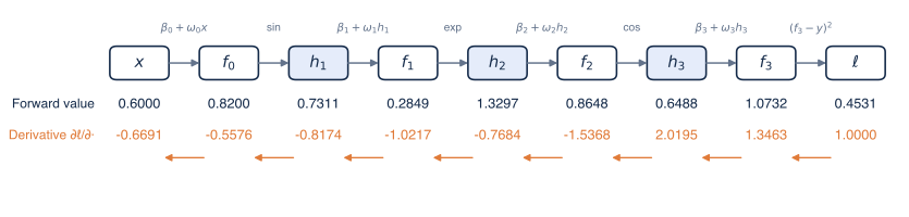
Figure 8.1 Forward and backward passes through a chain. The model of equation 8.2 with $x = 0.6$ and $y = 0.4$. The forward pass (dark arrows) applies each operation, shown above its arrow, and stores the result (dark numbers). The backward pass (orange arrows) starts from $\partial\ell/\partial\ell = 1$ and multiplies by one local derivative per step (equation 8.3), giving the derivative of the loss with respect to every intermediate value (orange numbers).

The parameter derivatives now come almost for free. The bias $\beta_k$ enters only through $f_k$, with local derivative 1, and the weight $\omega_k$ enters through $f_k$ multiplied by $h_k$ (with $h_0 = x$):

$$\frac{\partial \ell}{\partial \beta_k} = \frac{\partial \ell}{\partial f_k}, \qquad \frac{\partial \ell}{\partial \omega_k} = h_k \frac{\partial \ell}{\partial f_k} \tag{8.4}$$

These are the two observations of section 1 in equation form. The weight's derivative is the derivative at the point where it acts, scaled by the activation it multiplies. For our values:

$k$	$\partial\ell/\partial\beta_k$	$\partial\ell/\partial\omega_k$
0	$-0.5576$	$0.6 \times (-0.5576) = -0.3346$
1	$-1.0217$	$0.7311 \times (-1.0217) = -0.7470$
2	$-1.5368$	$1.3297 \times (-1.5368) = -2.0434$
3	$1.3463$	$0.6488 \times 1.3463 = 0.8735$

Each of the eight values agrees with the central difference of equation 8.1, with $\epsilon = 10^{-6}$, to at least six decimal places. The backward pass needed about a dozen multiplications, roughly the work of one forward pass. The central differences needed sixteen forward passes.

3. The general rule: computational graphs

The chain had a single path from each value to the loss. Real networks branch: a hidden unit feeds every unit of the next layer, and a value can be used several times. The general rule handles this.

Any computation can be drawn as a computational graph: each node is a value, and an arrow from node $u$ to node $v$ means that $v$ is computed directly from $u$ (among other inputs). If $u$ is used by several nodes $v_1, \ldots, v_m$, a small change in $u$ changes all of them, and the effects on the loss add up. The multivariable chain rule gives:

$$\frac{\partial \ell}{\partial u} = \sum_{j=1}^{m} \frac{\partial v_j}{\partial u}\,\frac{\partial \ell}{\partial v_j} \tag{8.5}$$

We can break this down into two parts. The derivatives $\partial\ell/\partial v_j$ belong to nodes later in the graph and are already known if we process nodes from the loss backwards. The factors $\partial v_j / \partial u$ are local: each depends only on the single operation that computes $v_j$, evaluated at the stored forward values. In words: the derivative of the loss with respect to a value is the sum, over everything that uses the value, of that user's derivative times the local derivative.

A tiny example shows the summation. Let $u = 3$ feed two operations, $v_1 = 2u = 6$ and $v_2 = u^2 = 9$, and let $\ell = v_1 + v_2 = 15$. Then $\partial\ell/\partial v_1 = \partial\ell/\partial v_2 = 1$, and equation 8.5 gives $\partial\ell/\partial u = 2 \times 1 + 2u \times 1 = 8$. Writing the loss directly as $\ell = 2u + u^2$ gives the same derivative, $2 + 2u = 8$. Forgetting one of the paths, a common bug in hand-written gradients, would give 2 or 6.

The algorithm is then: run the forward pass, storing every node's value; set $\partial\ell/\partial\ell = 1$; visit the nodes in reverse order of computation, and for each node apply equation 8.5. Every arrow of the graph is used once in each direction, so the backward pass costs a small constant multiple of the forward pass, however many parameters there are. That is the whole of backpropagation. The rest of this article specializes it to deep networks and examines its consequences.

4. Backpropagation in matrix form

We now apply the general rule to the deep network of article 7 (equation 7.4). It is convenient to name the pre-activations. With $\mathbf{h}_0 = \mathbf{x}$, the forward pass computes, for $k = 0, \ldots, K$:

$$\mathbf{f}_k = \boldsymbol{\beta}_k + \boldsymbol{\Omega}_k \mathbf{h}_k, \qquad \mathbf{h}_{k+1} = a(\mathbf{f}_k) \ \ (k < K) \tag{8.6}$$

and the output is $\mathbf{f}_K$. We define the error signal of layer $k$ as the derivative of the loss with respect to that layer's pre-activations, $\boldsymbol{\delta}_k = \partial\ell/\partial\mathbf{f}_k$, a vector with $D_{k+1}$ elements.

Parameters. Element $d$ of $\mathbf{f}_k$ is $f_{k,d} = \beta_{k,d} + \sum_j \Omega_{k,dj} h_{k,j}$. The weight $\Omega_{k,dj}$ appears only in this element, multiplied by $h_{k,j}$, so $\partial\ell/\partial\Omega_{k,dj} = \delta_{k,d}\,h_{k,j}$, exactly as in equation 8.4. Collecting all $d$ and $j$:

$$\frac{\partial \ell}{\partial \boldsymbol{\beta}_k} = \boldsymbol{\delta}_k, \qquad \frac{\partial \ell}{\partial \boldsymbol{\Omega}_k} = \boldsymbol{\delta}_k \mathbf{h}_k^\top \tag{8.7}$$

The weight gradient is an outer product: a column vector with $D_{k+1}$ elements times a row vector with $D_k$ elements, which gives a $D_{k+1} \times D_k$ matrix, the same shape as $\boldsymbol{\Omega}_k$. In words: the gradient for the weight from unit $j$ to unit $d$ is unit $d$'s error signal times unit $j$'s activation.

Moving back past a weight matrix. Unit $j$ of $\mathbf{h}_k$ is used by every element of $\mathbf{f}_k$, with local derivative $\partial f_{k,d}/\partial h_{k,j} = \Omega_{k,dj}$. Equation 8.5 sums over these uses: $\partial\ell/\partial h_{k,j} = \sum_d \Omega_{k,dj}\,\delta_{k,d}$. The sum runs down column $j$ of $\boldsymbol{\Omega}_k$, so in matrix form it is a product with the transpose:

$$\frac{\partial \ell}{\partial \mathbf{h}_k} = \boldsymbol{\Omega}_k^\top \boldsymbol{\delta}_k \tag{8.8}$$

The shapes check: $(D_k \times D_{k+1})$ times $D_{k+1}$ elements gives $D_k$ elements, one per unit of $\mathbf{h}_k$. The forward pass multiplies by $\boldsymbol{\Omega}_k$; the backward pass multiplies by $\boldsymbol{\Omega}_k^\top$ and sends each error signal back along the same connections.

Moving back past the activation. Element $j$ of $\mathbf{h}_k$ depends only on element $j$ of $\mathbf{f}_{k-1}$, so the local derivative is the slope of the activation function there:

$$\boldsymbol{\delta}_{k-1} = a'(\mathbf{f}_{k-1}) \odot \frac{\partial \ell}{\partial \mathbf{h}_k} \tag{8.9}$$

where $\odot$ multiplies two vectors element by element. For ReLU, the slope is 1 where the pre-activation is positive and 0 where it is negative, so equation 8.9 zeroes the error signal of every inactive unit. (At exactly zero the derivative is undefined; libraries use 0.)

Together, equations 8.7–8.9 are the backward pass for a deep network:

1. Run the forward pass (equation 8.6), storing every $\mathbf{h}_k$ and $\mathbf{f}_k$ (for ReLU, the signs of $\mathbf{f}_k$ are enough).
2. Compute $\boldsymbol{\delta}_K = \partial\ell/\partial\mathbf{f}_K$ from the loss (section 6).
3. For $k = K, K-1, \ldots, 0$: compute the parameter gradients of layer $k$ with equation 8.7; if $k > 0$, compute $\boldsymbol{\delta}_{k-1}$ with equations 8.8 and 8.9.

We work through a network with sizes $(2, 2, 2, 1)$, which has 15 parameters, ReLU activations and squared error. The input is $\mathbf{x} = (1, 2)^\top$, the target is $y = 1$, and the parameters are:

$$\boldsymbol{\Omega}_0 = \begin{bmatrix} 1 & -1 \\ 0.5 & 1 \end{bmatrix},\ \boldsymbol{\beta}_0 = \begin{bmatrix} 0 \\ -1 \end{bmatrix},\quad \boldsymbol{\Omega}_1 = \begin{bmatrix} 1 & 2 \\ -1 & -1 \end{bmatrix},\ \boldsymbol{\beta}_1 = \begin{bmatrix} 0.5 \\ 0 \end{bmatrix},\quad \boldsymbol{\Omega}_2 = \begin{bmatrix} 0.5 & -1 \end{bmatrix},\ \boldsymbol{\beta}_2 = 0.5$$

The forward pass gives $\mathbf{f}_0 = (1 - 2,\ -1 + 0.5 + 2) = (-1, 1.5)$, so $\mathbf{h}_1 = (0, 1.5)$: the first unit of layer 1 is inactive. Then $\mathbf{f}_1 = (0.5 + 3,\ -1.5) = (3.5, -1.5)$ and $\mathbf{h}_2 = (3.5, 0)$: the second unit of layer 2 is inactive. The output is $f_2 = 0.5 + 0.5 \times 3.5 = 2.25$ and the loss is $(2.25 - 1)^2 = 1.5625$.

The backward pass starts with $\delta_2 = 2(2.25 - 1) = 2.5$. Equation 8.7 gives $\partial\ell/\partial\boldsymbol{\Omega}_2 = 2.5 \times (3.5, 0) = (8.75, 0)$. Equation 8.8 gives $\partial\ell/\partial\mathbf{h}_2 = \boldsymbol{\Omega}_2^\top \times 2.5 = (1.25, -2.5)$, and equation 8.9 zeroes the inactive second element: $\boldsymbol{\delta}_1 = (1.25, 0)$. One layer further back:

$$\frac{\partial \ell}{\partial \boldsymbol{\Omega}_1} = \begin{bmatrix} 1.25 \\ 0 \end{bmatrix} \begin{bmatrix} 0 & 1.5 \end{bmatrix} = \begin{bmatrix} 0 & 1.875 \\ 0 & 0 \end{bmatrix}, \qquad \frac{\partial \ell}{\partial \mathbf{h}_1} = \boldsymbol{\Omega}_1^\top \begin{bmatrix} 1.25 \\ 0 \end{bmatrix} = \begin{bmatrix} 1.25 \\ 2.5 \end{bmatrix}$$

and zeroing the inactive first unit gives $\boldsymbol{\delta}_0 = (0, 2.5)$, so $\partial\ell/\partial\boldsymbol{\Omega}_0 = \boldsymbol{\delta}_0\mathbf{x}^\top$ has rows $(0, 0)$ and $(2.5, 5)$. All 15 derivatives agree with central differences. Figure 8.2 shows the values on the network.

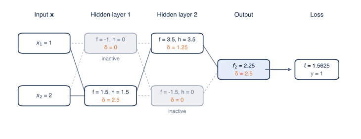
Figure 8.2 Backpropagation through a small ReLU network. Sizes $(2, 2, 2, 1)$, input $\mathbf{x} = (1, 2)$, target $y = 1$, parameters as in section 4. Each unit shows its pre-activation $f$ and activation $h$ from the forward pass (dark) and its error signal $\delta = \partial\ell/\partial f$ from the backward pass (orange). The gray units are inactive ($f < 0$): they pass nothing forward, their error signal is zero, and every weight into or out of them gets a zero gradient for this example (dashed lines).

The example shows two properties that hold in general. First, an inactive ReLU unit blocks the gradient for this example in both directions: its incoming weights get $\delta = 0$ and its outgoing weights multiply $h = 0$. A unit that is inactive for every training example never changes, which is called a dead ReLU. Second, each example's weight gradient $\boldsymbol{\delta}_k\mathbf{h}_k^\top$ has rank one. The gradient over a batch, a sum of such outer products, usually has higher rank, but at most the batch size.

5. Batches, cost and memory

Training uses a batch of $B$ examples and the mean loss $L = \frac{1}{B}\sum_i \ell_i$ (article 5). Each example has its own forward and backward pass, and the gradient of $L$ is the mean of the per-example gradients. With the activations of the batch as columns, $\mathbf{H}_k \in \mathbb{R}^{D_k \times B}$ as in article 7, and the error signals as columns of $\boldsymbol{\Delta}_k \in \mathbb{R}^{D_{k+1} \times B}$, the sum over examples of the outer products in equation 8.7 is one matrix product:

$$\frac{\partial L}{\partial \boldsymbol{\Omega}_k} = \frac{1}{B}\,\boldsymbol{\Delta}_k \mathbf{H}_k^\top, \qquad \frac{\partial L}{\partial \boldsymbol{\beta}_k} = \frac{1}{B}\,\boldsymbol{\Delta}_k \mathbf{1} \tag{8.10}$$

The shapes are $(D_{k+1} \times B)(B \times D_k) = D_{k+1} \times D_k$: the product sums over the batch dimension. Equation 8.8 becomes $\boldsymbol{\Omega}_k^\top\boldsymbol{\Delta}_k$, one product for the whole batch.

Operations. Per layer, the forward pass does one matrix product, $\boldsymbol{\Omega}_k\mathbf{H}_k$, with $D_{k+1} D_k B$ multiply-adds. The backward pass does two of the same size: $\boldsymbol{\Delta}_k\mathbf{H}_k^\top$ for the weight gradient and $\boldsymbol{\Omega}_k^\top\boldsymbol{\Delta}_k$ to continue backwards. The first layer can skip the second product, because nothing needs $\partial\ell/\partial\mathbf{x}$. So the backward pass costs about twice the forward pass, and a training step about three times. For the $(784, 256, 256, 10)$ classifier, the forward pass needs 268,800 multiply-adds per example and the backward pass 336,896; the ratio is only 1.25 because the large first layer skips its second product.

Memory. Equation 8.10 needs $\mathbf{H}_k$, and equation 8.9 needs the signs of $\mathbf{f}_{k-1}$, both from the forward pass. Training must therefore keep every layer's activations for the whole batch until the backward pass reaches that layer, which costs memory proportional to $B \sum_k D_k$. At prediction time there is no backward pass, and each layer's activations can be discarded once the next layer is computed. This is why training needs much more memory than prediction, and why the batch size is often limited by memory. Gradient checkpointing [7] trades computation for memory: it stores the activations of only some layers and recomputes the others during the backward pass, which for a chain of $K$ layers reduces activation memory to about $\sqrt{K}$ layers' worth at the cost of roughly one extra forward pass.

6. Starting the backward pass: the loss

The backward pass starts from $\boldsymbol{\delta}_K = \partial\ell/\partial\mathbf{f}_K$, which depends on the loss.

Squared error. For $\ell = \sum_k (f_{K,k} - y_k)^2$, the derivative is $\boldsymbol{\delta}_K = 2(\mathbf{f}_K - \mathbf{y})$: the error itself, doubled. If the loss is a mean over $I$ examples, each example's signal is divided by $I$.

Softmax and cross-entropy. For classification, the network outputs scores $\mathbf{z} = \mathbf{f}_K$, softmax turns them into probabilities $p_k = e^{z_k}/\sum_j e^{z_j}$, and the loss is $\ell = -\log p_c$ for the correct class $c$ (article 4). Substituting the softmax and using $\log(e^{z_c}) = z_c$:

$$\ell = -z_c + \log \sum_{j} e^{z_j}$$

where $j$ runs over all classes. The first term depends only on $z_c$, with derivative $-1$ for $k = c$ and 0 otherwise. The derivative of the second term with respect to $z_k$ is $e^{z_k}/\sum_j e^{z_j} = p_k$. Together:

$$\frac{\partial \ell}{\partial z_k} = p_k - \mathbb{1}[k = c] \tag{8.11}$$

where $\mathbb{1}[k = c]$ is 1 for the correct class and 0 otherwise. In words: the error signal is the predicted probability minus the target probability. For the scores of article 4, $\mathbf{z} = (2.0, 0.5, -1.0)$ with probabilities $(0.786, 0.175, 0.039)$, and the photograph showing a cat, the error signal is $(-0.214, 0.175, 0.039)$. Gradient descent moves against it: it raises the cat score and lowers the other two, each in proportion to how wrong its probability is. The elements always sum to zero, because the probabilities sum to 1.

Equation 8.11 is simpler and better behaved than the two steps taken separately. Computing $p_c$ first and then $-\log p_c$ fails when $p_c$ underflows to zero in floating point, and the derivative of $-\log p$ alone, $-1/p$, is huge exactly where the softmax's own derivative is tiny. Libraries therefore provide a fused "cross-entropy from scores" that computes $\log\sum_j e^{z_j}$ as $m + \log\sum_j e^{z_j - m}$ with $m = \max_j z_j$, so no exponential overflows, and uses equation 8.11 for the backward pass.

7. Automatic differentiation

Nothing in sections 3–6 is specific to neural networks. Any program built from operations whose local derivatives are known (additions, products, matrix products, exponentials, ReLU and so on) defines a computational graph, and the backward pass of section 3 computes the derivative of its output with respect to all of its inputs. This is reverse-mode automatic differentiation, and backpropagation is its special case for neural networks. Libraries such as PyTorch and JAX record the operations as the forward pass runs (or trace the program in advance) and provide, for each primitive operation, a rule that maps the derivative with respect to its output to the derivatives with respect to its inputs. Users write only the forward computation.

It helps to see why the reverse direction is the right one. For a chain of layers, the chain rule writes the gradient as a product of Jacobian matrices, $\partial\ell/\partial\mathbf{x}^\top = \partial\ell/\partial\mathbf{f}_K^\top\,\mathbf{J}_K \cdots \mathbf{J}_1$, where $\mathbf{J}_k$ is the matrix of derivatives of layer $k$'s outputs with respect to its inputs. The leftmost factor is a row vector, because the loss is a single number. Multiplying from the left keeps every intermediate result a vector, and each step costs a vector-matrix product. Multiplying from the right instead carries full matrices through the chain. Forward-mode automatic differentiation does the latter one column at a time: it pushes the derivative with respect to one input forward alongside the values, which needs one pass per input or parameter. For a scalar loss and many parameters, reverse mode costs a small constant multiple of one forward pass, independent of the number of parameters [5]; forward mode costs a multiple of the number of parameters. Forward mode wins in the opposite situation, few inputs and many outputs.

Hand-written or custom gradients should be checked against central differences (equation 8.1). The central difference has error proportional to $\epsilon^2$, against $\epsilon$ for the one-sided version. In 64-bit arithmetic, $\epsilon$ around $10^{-6}$ and a relative error below about $10^{-6}$ between the two gradients are typical; 32-bit arithmetic is too imprecise for a reliable check. Points within $\epsilon$ of a ReLU kink can disagree for a legitimate reason, because the two evaluations land on different linear pieces.

8. What the backward pass says about training deep networks

Unrolling equations 8.8 and 8.9 from the output to the first layer shows the structure of the error signal:

$$\boldsymbol{\delta}_0 = a'(\mathbf{f}_0) \odot \boldsymbol{\Omega}_1^\top \Big( a'(\mathbf{f}_1) \odot \boldsymbol{\Omega}_2^\top \big( \cdots \big( a'(\mathbf{f}_{K-1}) \odot \boldsymbol{\Omega}_K^\top \boldsymbol{\delta}_K \big) \cdots \big) \Big) \tag{8.12}$$

The signal that reaches an early layer has been multiplied by one weight matrix and one activation slope per layer. Products of many factors tend to grow or shrink exponentially with their length, and the same is true of the forward pass, which multiplies by one weight matrix and one activation per layer. The size of the weights decides which happens. This is the reason behind the initialization rule that article 5 stated without proof, and we can now derive it.

Forward. Suppose the weights of layer $k$ are drawn independently with mean 0 and variance $\sigma^2$, the biases are 0, and the pre-activations of the previous layer are symmetric around zero. Element $d$ of $\mathbf{f}_k$ is a sum of $D_k$ independent terms $\Omega_{k,dj}h_{k,j}$, each with mean 0 and variance $\sigma^2\,\mathbb{E}[h_{k,j}^2]$. A ReLU of a symmetric variable keeps exactly half of its squared mass, so $\mathbb{E}[h_{k,j}^2] = \frac{1}{2}\mathrm{Var}(f_{k-1,j})$. Hence:

$$\mathrm{Var}(f_k) = \frac{D_k\,\sigma^2}{2}\,\mathrm{Var}(f_{k-1}) \tag{8.13}$$

Backward. Element $j$ of equation 8.8 is a sum of $D_{k+1}$ terms $\Omega_{k,dj}\delta_{k,d}$, and equation 8.9 keeps about half of the results. Treating the weights, error signals and activation pattern as independent (an approximation, but a good one at initialization), the same argument gives:

$$\mathrm{Var}(\delta_{k-1}) = \frac{D_{k+1}\,\sigma^2}{2}\,\mathrm{Var}(\delta_k) \tag{8.14}$$

In words: each layer multiplies the variance of the forward signal by $D_k\sigma^2/2$ and the variance of the backward signal by $D_{k+1}\sigma^2/2$. If these factors are smaller than 1, both signals vanish exponentially with depth; if they are larger, both explode. They equal 1 when $\sigma^2 = 2/D_k$ (forward) or $\sigma^2 = 2/D_{k+1}$ (backward), which is He initialization [6]. When all hidden layers have the same width $D$, both conditions say $\sigma^2 = 2/D$.

Figure 8.3 checks this with a simulation: 50 ReLU layers of width 100, no biases, a batch of 256 random inputs, weights with variance $c/D$ for $c = 1, 2, 3$, and a random error signal at the top. With $c = 2$, the pre-activations and error signals keep roughly the same size through all 50 layers. With $c = 1$, each layer multiplies the standard deviation by about $\sqrt{1/2}$: after 50 layers the pre-activations have shrunk to $1.45 \times 10^{-8}$ of their size, and the error signal at the first layer to $1.58 \times 10^{-8}$. With $c = 3$, both grow by about $\sqrt{3/2}$ per layer, to $2.9 \times 10^{4}$ and $1.6 \times 10^{4}$.

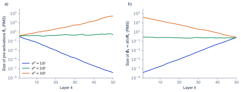
Figure 8.3 The scale of the initial weights decides whether signals survive 50 layers. A ReLU network with 50 layers of width 100, weights drawn with variance $\sigma^2 = c/D$, a batch of 256 random inputs and a random error signal at the last layer. a) The root-mean-square size of the pre-activations $\mathbf{f}_k$ in the forward pass. b) The size of the error signals $\boldsymbol{\delta}_k$ in the backward pass, which runs from layer 50 down to layer 1. With $c = 2$ (green, He initialization) both stay near 1, as equations 8.13 and 8.14 predict. With $c = 1$ (blue) both shrink by a factor of about $\sqrt{2}$ per layer, and with $c = 3$ (orange) both grow by about $\sqrt{1.5}$ per layer.

A subtlety appears when we look at the weight gradients themselves. By equation 8.7, the gradient of layer $k$ is $\boldsymbol{\delta}_k\mathbf{h}_k^\top$. With $c = 1$, the activations are small in late layers and the error signals are small in early layers, and the product is small in every layer by about the same overall factor, $(c/2)^{K/2} \approx 3 \times 10^{-8}$; the simulation measures weight-gradient norms between $5 \times 10^{-8}$ and $10^{-7}$ at layers 1, 25 and 50 alike. So in a plain ReLU network with equal widths, a bad scale does not make early layers learn more slowly than late ones. It makes the whole network's outputs and gradients useless, and no single learning rate fixes outputs that are $10^{-8}$ times the size they should be. In other settings the imbalance between layers is real. With sigmoid or tanh units, whose slopes are below 1 almost everywhere, and in recurrent networks, which multiply by the same matrix at every time step, the error signals shrink on the way back while the activations do not, so early layers or early time steps receive tiny gradients. This is the vanishing gradient problem in its classic form [8].

Initialization keeps the signals the right size at the start of training. It does not keep them there as the weights change, and it does not help with a different difficulty: the deep plain network that trains worse than a shallow one (article 7, section 5). Article 11 introduces residual connections, which add an identity path to every layer so that equation 8.12 no longer consists only of products, and normalization layers, which reset the scale of the activations at every layer.

Summary

Backpropagation computes the derivative of the loss with respect to every parameter in one backward pass whose cost is a small multiple of the forward pass. The forward pass stores the intermediate values. The backward pass starts from the derivative of the loss and visits the values in reverse order, multiplying by one local derivative per operation and summing over every use of a value (equation 8.5). For a deep network this gives three equations: the weight gradient is the error signal times the activation it multiplies, an outer product; the error signal moves back past a weight matrix by multiplying with its transpose; and it moves back past ReLU by zeroing inactive units. The backward pass costs about twice the forward pass, and training must keep every layer's activations, which is why it needs much more memory than prediction. For softmax with cross-entropy, the backward pass starts from the predicted probabilities minus the targets. The same algorithm, applied to any program, is reverse-mode automatic differentiation. Finally, the backward pass is a product of one factor per layer, and analysing its variance gives He initialization; the remaining difficulties of training very deep networks are taken up in article 11. Article 9 now turns from fitting the training data to generalizing beyond it.

Notes

History. Reverse-mode differentiation was described by Linnainmaa in 1970 [3] as a way to compute the rounding errors of long computations, and Werbos proposed applying it to neural networks in his 1974 thesis [4]. Rumelhart, Hinton and Williams [2] showed in 1986 that it lets multilayer networks learn useful internal representations, and that paper brought it into wide use. Baydin and colleagues [9] survey automatic differentiation for machine learning.

Second derivatives. Backpropagation gives the gradient. Second derivatives, the Hessian matrix, have $P^2$ entries and are rarely formed for neural networks. Products of the Hessian with a vector can be computed at the cost of a few gradient evaluations by applying forward mode to the backward pass, which is how many analyses of the loss curvature work.

Other initializations. For activations that are linear near zero, such as tanh, equation 8.13 without the factor $1/2$ suggests $\sigma^2 = 1/D$. Glorot and Bengio [10] compromised between the forward and backward conditions with $\sigma^2 = 2/(D_k + D_{k+1})$, often called Xavier initialization. The derivations assume independent weights; orthogonal initialization, which draws each weight matrix as a random rotation, preserves the length of every vector exactly in a linear network.

Non-differentiable points. ReLU has no derivative at 0, and maximum and absolute-value operations have similar kinks. Automatic differentiation picks one value of the derivative there (for ReLU, 0). Because pre-activations are exactly zero with negligible probability, this choice rarely matters in practice.

Reading further. Chapter 7 of Understanding Deep Learning [1] derives backpropagation for the same toy model and for deep networks, and covers initialization. Griewank and Walther [5] is the standard reference on automatic differentiation.

Problems

Problem 8.1 For the chain of section 2, compute $\partial\ell/\partial x$. Why does training never need it? (Answer: $\omega_0\,\partial\ell/\partial f_0 = 1.2 \times (-0.5576) = -0.6691$. The input is data, not a parameter, so gradient descent never updates it.)

Problem 8.2 In the network of section 4, change the target to $y = 3$ and leave everything else unchanged. What are the new gradients? (Answer: the forward pass is unchanged and $\delta_2 = 2(2.25 - 3) = -1.5$. Every gradient is linear in $\delta_2$, so all of them are multiplied by $-1.5/2.5 = -0.6$: for example $\partial\ell/\partial\boldsymbol{\Omega}_2 = (-5.25, 0)$ and $\partial\ell/\partial\boldsymbol{\Omega}_0$ has rows $(0, 0)$ and $(-1.5, -3)$.)

Problem 8.3 For the scores $\mathbf{z} = (2.0, 0.5, -1.0)$, compute the error signal of equation 8.11 when the correct class is the second one. Show that the elements of equation 8.11 always sum to zero. (Answer: $(0.786, -0.825, 0.039)$. The sum is $\sum_k p_k - 1 = 0$.)

Problem 8.4 Let $u = 1$, $v_1 = 2u$, $v_2 = u^2$ and $\ell = v_1 v_2$. Compute $\partial\ell/\partial u$ with equation 8.5 and check it by writing $\ell$ as a function of $u$. (Answer: $\partial\ell/\partial v_1 = v_2 = 1$ and $\partial\ell/\partial v_2 = v_1 = 2$, so $\partial\ell/\partial u = 2 \times 1 + 2u \times 2 = 6$. Directly, $\ell = 2u^3$ and its derivative is $6u^2 = 6$.)

Problem 8.5 How many multiply-adds does one training step of the $(784, 256, 256, 10)$ classifier need for a batch of 256, forward and backward together? (Answer: $256 \times (268{,}800 + 336{,}896) = 155{,}058{,}176$, about 155 million.)

Problem 8.6 Repeat the forward-variance derivation of section 8 for an activation function that is the identity, $a(z) = z$. Which weight variance keeps the pre-activations the same size? (Answer: without the ReLU, $\mathbb{E}[h^2] = \mathrm{Var}(f)$, so $\mathrm{Var}(f_k) = D_k\sigma^2\,\mathrm{Var}(f_{k-1})$ and $\sigma^2 = 1/D_k$.)

Problem 8.7 In the simulation of figure 8.3 with $c = 1$, by roughly what factor should the size of the pre-activations shrink between layer 1 and layer 50, according to equation 8.13? Compare with the measured $0.988$ and $1.45 \times 10^{-8}$. (Answer: $(1/2)^{49/2} \approx 4.2 \times 10^{-8}$; the measured ratio is $1.47 \times 10^{-8}$, the same order of magnitude. The difference comes from random fluctuations that compound over 49 layers.)

References

• 1: Simon J.D. Prince (2023). Understanding Deep Learning. MIT Press.
• 2: David Rumelhart, Geoffrey Hinton and Ronald Williams (1986). Learning representations by back-propagating errors. Nature 323, 533–536.
• 3: Seppo Linnainmaa (1970). The representation of the cumulative rounding error of an algorithm as a Taylor expansion of the local rounding errors. Master's thesis, University of Helsinki.
• 4: Paul Werbos (1974). Beyond regression: new tools for prediction and analysis in the behavioral sciences. PhD thesis, Harvard University.
• 5: Andreas Griewank and Andrea Walther (2008). Evaluating Derivatives: Principles and Techniques of Algorithmic Differentiation, 2nd edition. SIAM.
• 6: Kaiming He, Xiangyu Zhang, Shaoqing Ren and Jian Sun (2015). Delving deep into rectifiers: surpassing human-level performance on ImageNet classification. International Conference on Computer Vision.
• 7: Tianqi Chen, Bing Xu, Chiyuan Zhang and Carlos Guestrin (2016). Training deep nets with sublinear memory cost. arXiv:1604.06174.
• 8: Yoshua Bengio, Patrice Simard and Paolo Frasconi (1994). Learning long-term dependencies with gradient descent is difficult. IEEE Transactions on Neural Networks 5(2), 157–166.
• 9: Atılım Güneş Baydin, Barak Pearlmutter, Alexey Radul and Jeffrey Siskind (2018). Automatic differentiation in machine learning: a survey. Journal of Machine Learning Research 18(153), 1–43.
• 10: Xavier Glorot and Yoshua Bengio (2010). Understanding the difficulty of training deep feedforward neural networks. International Conference on Artificial Intelligence and Statistics.