Regularization: fitting less to generalize better

Article 6 showed that a flexible model can fit the noise in its training data and then predict badly, and it controlled this by choosing the model's complexity with a validation set: a polynomial of degree 3 instead of 9. For deep networks that tool is too blunt. Shrinking a network to the point where it cannot fit noise also stops it from fitting the patterns that matter, and in practice the best results come from networks large enough to memorize their training set. Regularization is the set of techniques that make such networks generalize anyway. This article works through the main ones on a single example: penalties on the size of the weights, stopping training early, averaging several models, dropout, adding noise and augmenting the data, and smoothing the labels. Each comes with a derivation of what it does in a case simple enough to solve exactly. The last part describes the overparameterized regime, where the classical picture of article 6 needs revising.

1. A network that overfits

We use one running example throughout. The data are 20 training points $(x_i, y_i)$ with $x_i$ drawn uniformly between 0 and 1 and $y_i = \sin(2\pi x_i) + \varepsilon_i$, where the noise $\varepsilon_i$ is normal with standard deviation 0.25. A validation set of 500 points comes from the same source. Because the noise has variance $0.25^2 = 0.0625$, even the true curve $\sin(2\pi x)$ has a validation error of about 0.0625. No model can do better on average, so 0.0625 is the floor for every number below.

The model is a fully connected ReLU network with sizes $(1, 64, 64, 1)$, which has 4,353 parameters (equation 7.5): more than 200 per training point. We train it to minimize the mean squared error

$$L(\boldsymbol{\phi}) = \frac{1}{I} \sum_{i=1}^{I} \big(f(x_i, \boldsymbol{\phi}) - y_i\big)^2 \tag{9.1}$$

with $I = 20$, using full-batch Adam [5] (article 5) with learning rate 0.003 for 30,000 steps, starting from He initialization. Every experiment in sections 2–5 uses this setup and changes one thing.

Without any regularization, the training error reaches 0.0091 and the validation error is 0.157 (figure 9.1a, orange). A training error far below the noise level of 0.0625 is the signature of overfitting: the network has fitted the particular noise values of the 20 points, and between them it bends in ways the true curve does not.

We call regularization any change to training that aims to reduce the error on new data rather than the error on the training data. Some regularizers change the loss (sections 2 and 6). Others change the training procedure (sections 3–5), and their effect on the solution is implicit.

2. L2 regularization and weight decay

The most common explicit regularizer adds the sum of the squared weights to the loss:

$$\tilde{L}(\boldsymbol{\phi}) = L(\boldsymbol{\phi}) + \lambda \sum_{k} \sum_{d,j} \Omega_{k,dj}^2 \tag{9.2}$$

We can break this down into two parts. The first term is the data loss of equation 9.1. The second is a penalty that grows with the size of the weights, summed over every entry of every weight matrix. The biases are usually left out: they shift the output and the activation thresholds but do not make the function steeper, and penalizing them would pull the outputs towards zero for no benefit. The regularization strength $\lambda \ge 0$ is a hyperparameter that trades the two terms against each other. In words: among parameter settings that fit the data about equally well, prefer the one with smaller weights.

The penalty's gradient with respect to a weight $\omega$ is $2\lambda\omega$, so one step of gradient descent with learning rate $\alpha$ becomes:

$$\omega \leftarrow (1 - 2\alpha\lambda)\,\omega - \alpha \frac{\partial L}{\partial \omega} \tag{9.3}$$

Every step first shrinks each weight by the factor $1 - 2\alpha\lambda$, then takes the usual gradient step. This is why L2 regularization is also called weight decay [4]. With $\alpha = 0.1$ and $\lambda = 0.01$, the factor is 0.998: a weight that received no gradient at all would decay to 13.5% of its value in 1,000 steps. Only weights that the data keep pushing on stay large.

Figure 9.1b shows the result of training our network with nine values of $\lambda$. Small values change little. As $\lambda$ grows, the training error rises, because the network can no longer bend freely enough to pass close to every noisy point, and the validation error falls. The best value in the sweep, $\lambda = 0.003$, has training error 0.0351 and validation error 0.0818, close to the floor of 0.0625. The fitted curve (figure 9.1a, blue) follows the sine and ignores the individual noise values. The weights are much smaller: the largest absolute weight is 1.54 instead of 8.03, and the sum of squared weights is 20.8 instead of 566.7. Beyond $\lambda = 0.01$ the penalty dominates: at $\lambda = 0.1$ the network is pushed so close to zero weights that training and validation errors are both about 0.65, which is underfitting.

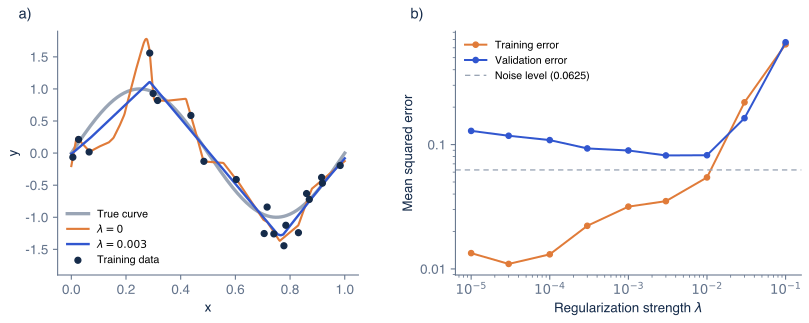
Figure 9.1 L2 regularization of a network with 4,353 parameters fitted to 20 points. a) The true curve (gray), the training data (dark points) and two trained networks: without regularization (orange), which bends to pass close to every point, and with $\lambda = 0.003$ (blue), which follows the trend. b) Training and validation error after 30,000 steps for $\lambda$ from $10^{-5}$ to $10^{-1}$. The dashed line is the noise variance, 0.0625, the lowest validation error any model can expect. Without regularization the errors are 0.0091 and 0.157.

TensorFlow Playground shows the same effect on a classification problem. The network below has three hidden layers of 8 ReLU units, 177 parameters in all, and is trained on a tenth of a noisy circle dataset; the other nine tenths are the test set.

Press play and watch the two loss curves above the output. Training loss keeps falling, but after about a hundred epochs test loss starts to rise. By epoch 800, training loss is around 0.2 or lower and test loss is above 0.4. The boundary sends thin arms out to reach individual training points. Then set Regularization rate to 0.03; the network restarts. Training loss now levels off higher, near 0.27, and test loss stays near 0.36 instead of climbing. Try 0.3 as well. The penalty dominates and both losses stay near 0.5: the network underfits, like the largest values of λ in figure 9.1b.

Open in TensorFlow Playground ↗

Why small weights mean a smoother function

The link between small weights and a well-behaved function can be made exact for ReLU networks. Inside one linear region, every ReLU acts as either 1 or 0, so for one input and one output the slope of the network is

$$\frac{\partial y}{\partial x} = \boldsymbol{\Omega}_K \mathbf{M}_{K-1} \boldsymbol{\Omega}_{K-1} \cdots \mathbf{M}_0 \boldsymbol{\Omega}_0$$

where $\mathbf{M}_k$ is a diagonal matrix with 1 for each active unit of layer $k+1$ and 0 for each inactive one. Multiplying by $\mathbf{M}_k$ can only shrink a vector, so the absolute slope is at most the product of the sizes of the weight matrices, $\prod_k \|\boldsymbol{\Omega}_k\|$ (using the largest factor by which each matrix can stretch a vector). A function that passes through noisy points spaced closely together needs steep pieces, and steep pieces need large weights. The penalty in equation 9.2 makes such weights expensive. This is a bound, not an equality: a network with large weights is not necessarily steep, but a steep network necessarily has large weights.

A probabilistic reading

L2 regularization also follows from treating the parameters as uncertain. Suppose the noise is normal with variance $\sigma^2$ and, before seeing data, we believe each weight is drawn from a normal distribution with mean 0 and variance $\sigma_\phi^2$, called the prior. The most probable weights given the data maximize the likelihood times the prior. Taking the negative logarithm and dropping terms that do not depend on the parameters gives

$$\frac{1}{2\sigma^2}\sum_{i=1}^{I}\big(f(x_i, \boldsymbol{\phi}) - y_i\big)^2 + \frac{1}{2\sigma_\phi^2}\sum \omega^2$$

and multiplying by $2\sigma^2/I$, which does not move the minimum, turns it into equation 9.2 with $\lambda = \sigma^2/(I\sigma_\phi^2)$. Two things follow. More data means a weaker penalty, because the data increasingly outweigh the prior. And $\lambda$ has a meaning: it is the noise variance relative to how large we expect the weights to be. For our data, $\sigma = 0.25$, $I = 20$ and a prior standard deviation of 1 give $\lambda = 0.0031$, close to the value the validation set chose. The prior width here is a guess, so the agreement should not be over-read. This estimate is called the maximum a posteriori (MAP) estimate.

Variants

Replacing the squares in equation 9.2 by absolute values gives L1 regularization, whose gradient has the same size for every nonzero weight and therefore drives many weights to exactly zero. It is used when a sparse model is wanted.

With adaptive optimizers such as Adam, equations 9.2 and 9.3 are no longer the same thing. Adam divides each parameter's gradient by a running estimate of its size, so the penalty gradient $2\lambda\omega$ is rescaled differently for each weight and large, frequently updated weights decay less than intended. Decoupled weight decay (AdamW) [6] applies the shrinking of equation 9.3 directly to the weights, outside the adaptive rescaling. It is the usual choice for training transformers. Our experiment used the penalty inside Adam, the simpler form.

3. Early stopping

Gradient descent does not jump to the minimum of the training loss; it moves towards it gradually, and the path matters. Figure 9.2a records the training and validation error of the unregularized network during its 30,000 steps. The training error keeps falling. The validation error falls until step 312, where the training error is 0.0327 and the validation error 0.0925, and then slowly rises to 0.157 as the network starts fitting the noise. Stopping at step 312 gives almost the same validation error as the best weight decay, without choosing $\lambda$.

Early stopping means exactly this: evaluate the validation error at regular intervals during training, keep a copy of the parameters with the lowest validation error so far, and stop when it has not improved for a while (a number of evaluations called the patience). The number of training steps becomes a hyperparameter that the validation set chooses, and it costs nothing extra to tune, because one training run visits every candidate value.

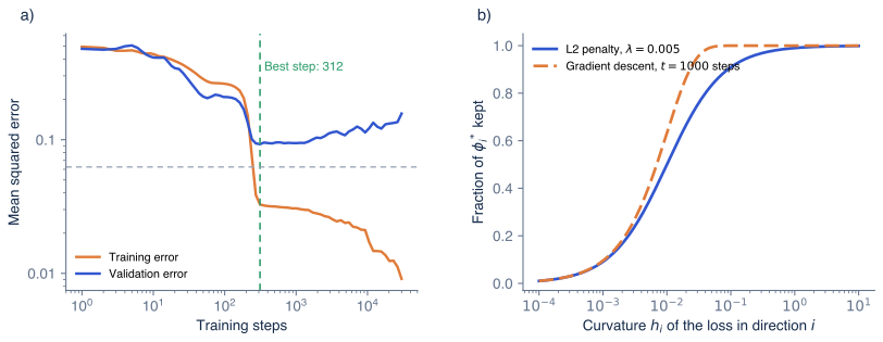
Figure 9.2 Early stopping. a) Training and validation error of the unregularized network during training. The validation error is lowest at step 312 (green), after which the network continues to reduce the training error by fitting noise. The dashed gray line is the noise level. b) For a quadratic loss, the fraction of each component of the minimum $\boldsymbol{\phi}^*$ that is kept by an L2 penalty with $\lambda = 0.005$ (equation 9.6) and by 1,000 steps of gradient descent from zero with $\alpha = 0.1$ (equation 9.5). Both keep components along directions of high curvature and suppress components along directions of low curvature, with nearly the same cutoff.

Early stopping as an L2 penalty

For a quadratic loss the connection to L2 regularization can be derived exactly. Near its minimum $\boldsymbol{\phi}^*$, write the loss as

$$L(\boldsymbol{\phi}) = L^* + \tfrac{1}{2}(\boldsymbol{\phi} - \boldsymbol{\phi}^*)^\top \mathbf{H}\,(\boldsymbol{\phi} - \boldsymbol{\phi}^*) \tag{9.4}$$

where $\mathbf{H}$ is the matrix of second derivatives, symmetric with eigenvalues $h_i \ge 0$ and eigenvectors $\mathbf{v}_i$. The eigenvalue $h_i$ is the curvature of the loss in direction $\mathbf{v}_i$: large where the data constrain the parameters tightly, small where moving the parameters barely changes the fit.

Gradient descent. The gradient is $\mathbf{H}(\boldsymbol{\phi} - \boldsymbol{\phi}^*)$, so the error $\mathbf{e}_t = \boldsymbol{\phi}_t - \boldsymbol{\phi}^*$ obeys $\mathbf{e}_{t+1} = (\mathbf{I} - \alpha\mathbf{H})\,\mathbf{e}_t$. Starting from $\boldsymbol{\phi}_0 = \mathbf{0}$, so $\mathbf{e}_0 = -\boldsymbol{\phi}^*$, the component of $\boldsymbol{\phi}_t$ along $\mathbf{v}_i$ after $t$ steps is:

$$\phi_{t,i} = \big[1 - (1 - \alpha h_i)^t\big]\,\phi^*_i \tag{9.5}$$

L2 penalty. Adding $\lambda\|\boldsymbol{\phi}\|^2$ to equation 9.4 and setting the gradient to zero gives $(\mathbf{H} + 2\lambda\mathbf{I})\boldsymbol{\phi} = \mathbf{H}\boldsymbol{\phi}^*$, so along $\mathbf{v}_i$:

$$\phi_i = \frac{h_i}{h_i + 2\lambda}\,\phi^*_i \tag{9.6}$$

Both equations multiply each component of the unregularized solution by a factor between 0 and 1. The factor is close to 1 where the curvature is high and close to 0 where it is low. For small $\alpha h_i$, $(1 - \alpha h_i)^t \approx e^{-\alpha h_i t}$, and the two factors switch from 0 to 1 at about the same curvature when $t \approx 1/(2\alpha\lambda)$. Figure 9.2b shows this for $\lambda = 0.005$, $\alpha = 0.1$ and $t = 1{,}000$. For example, along a direction with $h = 0.01$, the penalty keeps $0.01/(0.01 + 0.01) = 0.5$ of $\phi^*_i$ and gradient descent keeps $1 - 0.999^{1000} = 0.63$.

In words: training for fewer steps acts approximately like an L2 penalty whose strength is inversely proportional to the number of steps. The derivation assumes a quadratic loss, plain gradient descent and a start at zero. A network's loss is not quadratic and training starts from random weights, so the statement is qualitative there; but the mechanism, that the well-constrained directions are fitted first and the weakly constrained ones last, carries over and explains the shape of figure 9.2a.

4. Ensembles

A different way to reduce the error on new data is to train several models and average their predictions. The benefit comes from averaging away the parts of their errors that differ.

Suppose each of $M$ models makes an error $e_m$ at some input, with mean zero, variance $\sigma^2$, and correlation $\rho$ between any two models. The error of the average is $\bar{e} = \frac{1}{M}\sum_m e_m$, and its variance is

$$\mathrm{Var}(\bar{e}) = \frac{1}{M^2}\Big(\sum_m \mathrm{Var}(e_m) + \sum_{m \ne m'} \mathrm{Cov}(e_m, e_{m'})\Big) = \frac{1}{M^2}\big(M\sigma^2 + M(M-1)\rho\sigma^2\big) = \rho\sigma^2 + \frac{1 - \rho}{M}\sigma^2 \tag{9.7}$$

The first step expands the variance of a sum into variances and covariances; there are $M$ variances and $M(M-1)$ ordered pairs of distinct models, each with covariance $\rho\sigma^2$. In words: averaging removes the uncorrelated part of the errors, at a rate of $1/M$, and leaves the correlated part untouched. With $\rho = 0.5$ and $M = 5$, the variance falls to $0.6\sigma^2$; with $\rho = 0.8$, no number of models can bring it below $0.8\sigma^2$.

In our example, we trained five unregularized networks that differ only in their random initial weights. Their validation errors are 0.157, 0.204, 0.146, 0.174 and 0.134, with mean 0.163; the average of their predictions has validation error 0.139. Measured against the true curve, which removes the noise floor, the mean squared deviation falls from 0.089 for a single network to 0.065 for the ensemble. The five networks' deviations have an average correlation of 0.73, because all were trained on the same 20 points and fitted the same noise; equation 9.7 predicts a factor of $0.73 + 0.27/5 = 0.78$, giving 0.070, close to the measured 0.065 (the equation assumes equal variances and zero-mean errors, which hold only approximately).

The art of ensembling is reducing $\rho$. Networks can differ in their initialization, as here, in the order of the training examples, in their architecture, or in their training data. Bagging [7] trains each model on a bootstrap sample, $I$ examples drawn with replacement from the training set. Ensembles of independently initialized networks are among the most reliable ways to improve accuracy and to estimate the uncertainty of a prediction [8]. Their cost is $M$ times the computation at prediction time, which is often the reason not to use them.

5. Dropout

Dropout [3] approximates a huge ensemble at the cost of one network. At every training step, each hidden unit is independently set to zero with probability $p$, and the units that are kept are scaled up by $1/(1-p)$:

$$\tilde{\mathbf{h}} = \frac{1}{1 - p}\,\mathbf{m} \odot \mathbf{h}, \qquad m_j \sim \mathrm{Bernoulli}(1 - p) \tag{9.8}$$

Here $\mathbf{m}$ is a random mask of zeros and ones, drawn afresh for every example and every step, and $\mathrm{Bernoulli}(1-p)$ means "1 with probability $1 - p$, else 0". The scaling keeps the expected value unchanged, $\mathbb{E}[\tilde{h}_j] = h_j$, so that at prediction time we can use the whole network without a mask and the next layer receives inputs of the same average size. For example, with $p = 0.5$, the activations $\mathbf{h} = (0.8, 1.2, 0, 2.0)$ and the mask $(1, 0, 1, 1)$ give $\tilde{\mathbf{h}} = (1.6, 0, 0, 4.0)$. In the backward pass, the same mask and scale multiply the error signals, an extra factor in equation 8.9.

Our network trained with dropout on both hidden layers reaches validation errors of 0.113 for $p = 0.1$, 0.093 for $p = 0.3$ and 0.103 for $p = 0.5$, against 0.157 without. With $p = 0.5$ the training error is 0.067, no longer below the noise level.

Dropout as an ensemble. Each mask selects a subnetwork. Our network has 128 hidden units, so there are $2^{128}$ possible subnetworks, all sharing the same weights, and every training step trains a different random one. Using the full network with the expected activations at prediction time approximates averaging the predictions of all of them. The approximation is exact for a network with no nonlinearity after the dropped layer and only approximate otherwise. The original authors also argued that dropout prevents units from relying on particular other units being present ("co-adaptation"); that explanation is plausible but is a hypothesis, not a derivation.

Dropout as a penalty. For a linear model the effect can be computed exactly. Let the prediction be $f = \frac{1}{1-p}\sum_j w_j x_j m_j$ with dropout applied to the inputs. Its mean over masks is $\sum_j w_j x_j$, and since the masks are independent and $\mathrm{Var}(m_j/(1-p)) = p/(1-p)$, its variance is $\frac{p}{1-p}\sum_j w_j^2 x_j^2$. The expected squared error is the squared error of the mean plus the variance:

$$\mathbb{E}_{\mathbf{m}}\big[(f - y)^2\big] = \Big(\sum_j w_j x_j - y\Big)^2 + \frac{p}{1 - p}\sum_j w_j^2 x_j^2 \tag{9.9}$$

In words: on average, dropout trains the model without dropout plus an L2 penalty in which each weight is penalized in proportion to the squared size of the input it multiplies [9]. With $p = 0.5$, the factor $p/(1-p)$ is 1. Dropout is therefore a data-dependent form of weight decay, with the important difference that its penalty adapts to how large each input actually is.

Typical dropout rates are 0.1 to 0.5 for fully connected layers. It is used less in convolutional layers, whose units are strongly correlated with their neighbours, and transformers commonly use a small rate such as 0.1. Dropout interacts with batch normalization (article 11), because it changes the activation statistics between training and prediction.

6. Noise, data augmentation and label smoothing

Noise on the inputs. Adding random noise to the inputs during training is another implicit penalty. For a linear model with inputs $\tilde{\mathbf{x}} = \mathbf{x} + \boldsymbol{\epsilon}$, where the noise has mean zero and covariance $\sigma_\epsilon^2\mathbf{I}$, the same mean-plus-variance argument as for equation 9.9 gives

$$\mathbb{E}_{\boldsymbol{\epsilon}}\big[(\mathbf{w}^\top\tilde{\mathbf{x}} - y)^2\big] = (\mathbf{w}^\top\mathbf{x} - y)^2 + \sigma_\epsilon^2\,\|\mathbf{w}\|^2 \tag{9.10}$$

which is exactly L2 regularization with $\lambda$ proportional to $\sigma_\epsilon^2$ [10]. For a network the equivalence holds approximately, to first order in the noise, and the penalty is on the size of the derivative of the output with respect to the input: the network is discouraged from changing quickly as its input changes.

Data augmentation. Often we know transformations that do not change the correct output: a cat photograph flipped horizontally, cropped slightly, or made a little darker still shows a cat. Data augmentation applies random transformations of this kind to the training examples at every step, so that the network sees many versions of each. It encodes knowledge about the task that the data alone cannot supply, namely which changes the output should be insensitive to. For images, random crops and flips have been standard since the first large convolutional networks [11], and augmentation is usually the single most effective regularizer for vision models. The transformations must actually preserve the label: rotating a handwritten 6 by 180 degrees turns it into a 9, and flipping an image that contains text changes the text. A further step, mixup [12], trains on weighted averages of pairs of examples with the same weighted average of their labels.

Label smoothing. For classification with the cross-entropy loss, the target is a one-hot vector: probability 1 for the correct class. The loss approaches zero only as the correct class's score exceeds the others by an ever-growing margin, so training never stops pushing the scores apart, and the network becomes overconfident. Label smoothing [13] replaces the target with $\mathbf{t} = (1 - \epsilon)\,\text{one-hot} + \epsilon/K$, spreading a small amount $\epsilon$ of probability evenly over all $K$ classes. Repeating the derivation of equation 8.11 with this target gives the error signal $\mathbf{p} - \mathbf{t}$. For the scores of article 4, $\mathbf{z} = (2.0, 0.5, -1.0)$ with probabilities $(0.786, 0.175, 0.039)$, $\epsilon = 0.1$ and $K = 3$, the target is $(0.933, 0.033, 0.033)$ and the error signal is $(-0.148, 0.142, 0.006)$, smaller in the first element than the $-0.214$ of the one-hot target. The loss is now minimized at a finite score difference, where $\mathbf{p} = \mathbf{t}$.

7. Overparameterization and double descent

Our network has more than 200 parameters per training point, and even without regularization its validation error was 0.157: worse than with regularization, but not the catastrophe of the degree-9 polynomial of article 6. This is typical of modern deep learning, and the classical picture, in which more parameters than data points means hopeless overfitting, does not describe it. Zhang and colleagues [14] made the point sharply in 2017: standard image classification networks can fit CIFAR-10 perfectly even when every label is replaced by a random one, so they have the capacity to memorize anything, yet on the real labels the same networks generalize well. Counting parameters does not explain generalization.

A simple model shows what happens instead. Take a shallow network with $N$ hidden units whose first layer is fixed at random, with cosine activations: unit $n$ computes $\cos(\omega_n x + b_n)$ with a random frequency $\omega_n$ (normal, standard deviation 40) and a random phase $b_n$. Only the output layer, $N + 1$ weights including the bias, is trained, by least squares on our 20 points. The model is linear in its trainable weights, so the fit can be computed exactly. When $N + 1 > 20$, infinitely many weight vectors fit the 20 points exactly. We take the one with the smallest sum of squared weights, the minimum-norm solution. This is not an arbitrary choice: gradient descent on a least-squares loss, started from zero, converges to exactly this solution, because every gradient is a combination of the training inputs' feature vectors and so the weights never leave the space those vectors span, and the only exact fit within that space is the minimum-norm one.

Figure 9.3 shows the validation error as $N$ grows, the median over 60 random draws of the first layer. At first the curve has the classical U shape: the error falls from 0.70 with 2 units to 0.45 with 8, then rises as the model starts fitting noise. At $N + 1 = I = 20$ it reaches a peak of about 5,500. Then it falls again: 2.7 at $N = 60$, 0.30 at $N = 1{,}000$ and 0.297 at $N = 3{,}000$, below the minimum of the U. This second fall after the peak is called double descent [15].

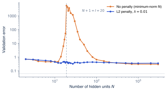
Figure 9.3 Double descent. Validation error of a shallow network with $N$ cosine hidden units whose first layer is random and fixed, with only the output weights fitted to the 20 training points; median over 60 draws of the first layer. Orange: no penalty, minimum-norm least squares. The error peaks where the number of trainable weights equals the number of training points ($N + 1 = 20$, dashed line) and falls again beyond it. Blue: an L2 penalty with $\lambda = 0.01$ removes the peak. The dotted line is the noise level.

The peak has a simple cause. At $N + 1 = I$ there is exactly one setting of the weights that fits all 20 points, and to pass through noisy values with only 20 fixed wave shapes it typically needs enormous weights that make the function swing wildly between the points. With fewer units there is no exact fit and least squares averages the noise; with more, there are many exact fits and the minimum-norm one is the gentlest. As $N$ grows, the set of exact fits grows and the gentlest among them becomes smoother. The training algorithm's built-in preference, here for small weights, does the regularizing. With an explicit penalty ($\lambda = 0.01$, blue) the peak disappears, which shows it is a symptom of an unregularized fit at the threshold rather than a property of the model size.

Nakkiran and colleagues [16] observed the same shape in deep networks trained in the usual way, as a function of width and also of the number of training epochs, and showed that suitable regularization can remove the peak. Some caveats keep the picture honest. Double descent is most visible with little or no regularization and noisy labels. The second descent does not always go below the first minimum; in our example it does (0.30 against 0.45), but both are far worse than the network of section 2 with weight decay (0.082), because random cosine features of a high frequency are a poor basis for a sine wave. And the implicit preferences of gradient descent in deep networks, unlike in this linear model, are not fully characterized; why heavily overparameterized networks generalize as well as they do remains an active research question.

8. Regularization in practice

The techniques combine, and practitioners rarely rely on one alone. A common recipe for a new problem is to start with a network large enough to fit the training set well, which confirms that the model and the training procedure work, and then add regularization until the validation error stops improving.

Technique	What it changes	Typical setting	Extra cost
Weight decay	Adds $\lambda\sum\omega^2$ to the loss, or shrinks weights each step	$\lambda$ from $10^{-5}$ to $10^{-1}$, depending on the optimizer; decoupled with Adam	None
Early stopping	Training length	Choose the step with the lowest validation error	Periodic validation
Data augmentation	Training examples	Task-specific label-preserving transformations	Data processing
Dropout	Hidden activations during training	$p$ from 0.1 to 0.5	Slower convergence
Label smoothing	Classification targets	$\epsilon = 0.1$	None
Ensembles	Predictions	3 to 10 models	$M$ times the computation

These ranges are common in published work, not rules; the right values depend on the data, the architecture and the optimizer, and they are chosen with the validation set, never the test set (article 6). Two architectural components introduced later also act as regularizers. Batch normalization (article 11) adds noise through its batch statistics. Convolutional layers (article 10) are the strongest regularizer of all for images: by sharing weights across positions, they rule out most of the functions a fully connected network could represent before training even starts.

Summary

A network with many more parameters than training examples can fit the noise in its data. Regularization changes the training so that it fits less of the noise. Weight decay adds a penalty on the squared weights, which bounds how steeply a ReLU network can change and corresponds to a normal prior on the weights. Early stopping halts training when the validation error is lowest; for a quadratic loss it is approximately equivalent to an L2 penalty whose strength falls as the number of steps grows, because gradient descent fits the well-constrained directions first. Ensembles average away the uncorrelated part of several models' errors, and dropout approximates an exponentially large ensemble of subnetworks; for a linear model, it is equivalent to a data-dependent L2 penalty. Input noise, data augmentation and label smoothing put knowledge or caution into the data and targets. Finally, highly overparameterized models can generalize because training prefers simple solutions among the many that fit, which produces the double descent of test error with model size. Article 10 turns to the strongest built-in regularizer for images, the convolutional layer.

Notes

Generalization theory. Classical bounds on the gap between training and test error depend on measures of model capacity such as the number of parameters, and they are far too loose to explain the generalization of large networks. Bounds based on the size of the weights (norm-based bounds), on how much the parameters can be perturbed without changing the loss (flatness, PAC-Bayes bounds) and on the compressibility of the trained network give tighter but still incomplete accounts. Chapter 9 of Understanding Deep Learning [1] reviews the evidence.

Implicit regularization of stochastic gradient descent. Training with small batches adds noise to each step, and there is evidence that this noise favours solutions in wide, flat regions of the loss, which tend to generalize better. The link between flatness and generalization is debated, because flatness depends on how the parameters are scaled.

Transfer learning. When the training set is small, the most effective regularizer is often to start from a network trained on a related, larger dataset and adapt it (fine-tuning). The pre-trained weights act as a strong prior. Pre-training on large unlabelled datasets is the basis of the language models introduced in article 12.

Reading further. Chapter 9 of Understanding Deep Learning [1] and chapter 7 of Goodfellow, Bengio and Courville [2] cover regularization, including the early-stopping analysis of section 3.

Problems

Problem 9.1 Using the MAP reading of section 2, what $\lambda$ corresponds to noise standard deviation 0.5, prior standard deviation 0.1 and 100 training examples? (Answer: $\lambda = 0.25/(100 \times 0.01) = 0.25$.)

Problem 9.2 With weight decay factor $1 - 2\alpha\lambda = 0.998$ and no gradient from the data, after how many steps has a weight halved? (Answer: $\ln 0.5 / \ln 0.998 \approx 346$.)

Problem 9.3 Ten models have errors with variance $\sigma^2$ and pairwise correlation 0.8. What is the variance of the error of their average? What is the limit as the number of models grows? (Answer: $0.8\sigma^2 + 0.2\sigma^2/10 = 0.82\sigma^2$; the limit is $0.8\sigma^2$.)

Problem 9.4 Apply inverted dropout with $p = 0.2$ to $\mathbf{h} = (2.0, 1.0, 0.5, 3.0)$ with the mask $(1, 1, 0, 1)$. (Answer: $(2.5, 1.25, 0, 3.75)$.)

Problem 9.5 Derive equation 9.10. (Hint: $\mathbf{w}^\top\tilde{\mathbf{x}} - y = (\mathbf{w}^\top\mathbf{x} - y) + \mathbf{w}^\top\boldsymbol{\epsilon}$; expand the square and use $\mathbb{E}[\boldsymbol{\epsilon}] = \mathbf{0}$ and $\mathbb{E}[(\mathbf{w}^\top\boldsymbol{\epsilon})^2] = \sigma_\epsilon^2\|\mathbf{w}\|^2$.)

Problem 9.6 With label smoothing $\epsilon = 0.1$ and $K = 10$ classes, what are the target probabilities? What is the smallest cross-entropy loss the model can reach on one example? (Answer: 0.91 for the correct class and 0.01 for each other class. The loss $-\sum_k t_k \log p_k$ is smallest when $\mathbf{p} = \mathbf{t}$, where it equals $-0.91\ln 0.91 - 9 \times 0.01\ln 0.01 \approx 0.500$.)

Problem 9.7 Using equations 9.5 and 9.6 with $\alpha = 0.1$, compare the fraction of $\phi^*_i$ kept along a direction with curvature $h = 0.01$ after 1,000 steps of gradient descent and with an L2 penalty $\lambda = 0.005$. (Answer: $1 - 0.999^{1000} \approx 0.632$ and $0.01/0.02 = 0.5$.)

References

• 1: Simon J.D. Prince (2023). Understanding Deep Learning. MIT Press.
• 2: Ian Goodfellow, Yoshua Bengio and Aaron Courville (2016). Deep Learning. MIT Press.
• 3: Nitish Srivastava, Geoffrey Hinton, Alex Krizhevsky, Ilya Sutskever and Ruslan Salakhutdinov (2014). Dropout: a simple way to prevent neural networks from overfitting. Journal of Machine Learning Research 15(56), 1929–1958.
• 4: Anders Krogh and John Hertz (1991). A simple weight decay can improve generalization. Advances in Neural Information Processing Systems 4.
• 5: Diederik Kingma and Jimmy Ba (2015). Adam: a method for stochastic optimization. International Conference on Learning Representations.
• 6: Ilya Loshchilov and Frank Hutter (2019). Decoupled weight decay regularization. International Conference on Learning Representations.
• 7: Leo Breiman (1996). Bagging predictors. Machine Learning 24(2), 123–140.
• 8: Balaji Lakshminarayanan, Alexander Pritzel and Charles Blundell (2017). Simple and scalable predictive uncertainty estimation using deep ensembles. Advances in Neural Information Processing Systems 30.
• 9: Stefan Wager, Sida Wang and Percy Liang (2013). Dropout training as adaptive regularization. Advances in Neural Information Processing Systems 26.
• 10: Chris Bishop (1995). Training with noise is equivalent to Tikhonov regularization. Neural Computation 7(1), 108–116.
• 11: Alex Krizhevsky, Ilya Sutskever and Geoffrey Hinton (2012). ImageNet classification with deep convolutional neural networks. Advances in Neural Information Processing Systems 25.
• 12: Hongyi Zhang, Moustapha Cisse, Yann Dauphin and David Lopez-Paz (2018). mixup: beyond empirical risk minimization. International Conference on Learning Representations.
• 13: Christian Szegedy, Vincent Vanhoucke, Sergey Ioffe, Jonathon Shlens and Zbigniew Wojna (2016). Rethinking the Inception architecture for computer vision. IEEE Conference on Computer Vision and Pattern Recognition.
• 14: Chiyuan Zhang, Samy Bengio, Moritz Hardt, Benjamin Recht and Oriol Vinyals (2017). Understanding deep learning requires rethinking generalization. International Conference on Learning Representations.
• 15: Mikhail Belkin, Daniel Hsu, Siyuan Ma and Soumik Mandal (2019). Reconciling modern machine-learning practice and the classical bias–variance trade-off. Proceedings of the National Academy of Sciences 116(32), 15849–15854.
• 16: Preetum Nakkiran, Gal Kaplun, Yamini Bansal, Tristan Yang, Boaz Barak and Ilya Sutskever (2020). Deep double descent: where bigger models and more data hurt. International Conference on Learning Representations.