Convolutional networks: learning the filters

Article 2 computed image features by sliding a small kernel, such as the Sobel edge kernel, across a photograph, and noted that every kernel had to be designed by hand. Article 3 counted the cost of the alternative, feeding the 135,300 pixels of that photograph into a fully connected layer: more than 13 million parameters for 100 hidden units. Article 9 claimed that convolutional layers are the strongest regularizer for images. This article explains all three. A convolutional layer is a fully connected layer with two restrictions, locality and weight sharing, which reduce its parameters from millions to hundreds and build in a property images have. Its weights are the kernels of article 2, but learned. We derive the layer from a one-dimensional example, extend it to images with several channels, follow how information from distant pixels reaches deep layers, assemble a complete classifier with its shapes and costs, and finally watch a kernel learn to become the Sobel filter.

1. Two properties of images

Two facts about images motivate the design. First, locality: whether a pixel lies on an edge, or on a cat's whisker, depends mostly on its neighbours, not on pixels on the other side of the image. Second, translation: a whisker looks the same wherever it appears, so a detector that works in the top-left corner should work everywhere.

A fully connected layer ignores both. Every hidden unit has its own weight for every pixel, so it must learn separately, from data, that distant pixels matter little and that a pattern means the same thing at every position. With 20 or even a million training images, much of that learning is wasted.

We can state the second property precisely. Let $t$ be a transformation of the input, such as shifting an image by a few pixels. A function $f$ is invariant to $t$ if $f(t(\mathbf{x})) = f(\mathbf{x})$: the output does not change. It is equivariant to $t$ if $f(t(\mathbf{x})) = t(f(\mathbf{x}))$: transforming the input transforms the output in the same way. An image classifier should be roughly invariant to shifts, because a shifted cat is still a cat. A layer that computes a feature map, such as edge strength at each pixel, should be equivariant, because when the cat moves, its edges should move with it. Convolution is exactly equivariant to shifts, as we show next.

2. Convolution in one dimension

We start with a one-dimensional input, such as a short audio signal, with six values $x_1, \ldots, x_6$. We defer images until section 4. A convolutional layer with a kernel of size 3 computes, at every position $i$:

$$z_i = \beta + \omega_1 x_{i-1} + \omega_2 x_i + \omega_3 x_{i+1} \tag{10.1}$$

We can break this down into three parts. The three weights $\omega_1, \omega_2, \omega_3$ are applied to the input at position $i$ and its two neighbours. A single bias $\beta$ is added. And the same four parameters are used at every position. At the ends, where $x_0$ and $x_7$ do not exist, we treat them as zero, which is called zero padding. In words: the layer slides one small weighted sum along the input, exactly like the kernel of article 2's equation 2.1. As in article 2, this is strictly a cross-correlation, but deep learning calls it convolution.

Take the input $\mathbf{x} = (0, 1, 3, 2, 0, 0)$, the kernel $\boldsymbol{\omega} = (-1, 0, 1)$ and $\beta = 0$. The kernel computes the difference between the right and left neighbours, the one-dimensional version of a Sobel row. At position 1 the output is $z_1 = x_2 - x_0 = 1$; at position 2, $z_2 = x_3 - x_1 = 3$; and so on, giving $\mathbf{z} = (1, 3, 1, -3, -2, 0)$ (figure 10.1a). The output is positive where the signal rises and negative where it falls. A ReLU after the layer, $\mathbf{h} = \mathrm{ReLU}(\mathbf{z}) = (1, 3, 1, 0, 0, 0)$, keeps only the rises: it is a detector for "increasing".

Now shift the input one place to the right, $\mathbf{x}' = (0, 0, 1, 3, 2, 0)$. The output is $\mathbf{z}' = (0, 1, 3, 1, -3, -2)$: the same values, shifted one place (figure 10.1b). This is equivariance, and it holds for any kernel, because every position uses the same weights. It is exact away from the ends; at the ends, padding with zeros breaks it slightly.

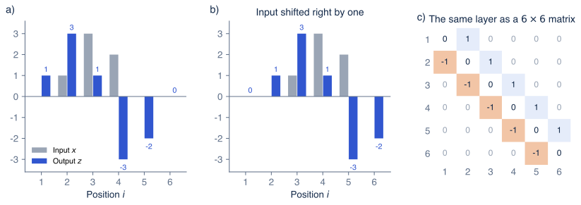
Figure 10.1 A one-dimensional convolution. a) The input $\mathbf{x} = (0, 1, 3, 2, 0, 0)$ (gray) and the output of equation 10.1 with kernel $(-1, 0, 1)$ and zero padding (blue): $\mathbf{z} = (1, 3, 1, -3, -2, 0)$. b) Shifting the input one position to the right shifts the output one position to the right. c) The same layer written as a fully connected layer: a $6 \times 6$ weight matrix whose entries are zero except on three diagonals, each of which repeats one kernel weight.

Convolution as a restricted fully connected layer

A fully connected layer from six inputs to six outputs computes $\mathbf{z} = \boldsymbol{\beta} + \boldsymbol{\Omega}\mathbf{x}$ with a $6 \times 6$ weight matrix, 36 weights and 6 biases. Equation 10.1 is a special case. Row $i$ of $\boldsymbol{\Omega}$ holds the weights that output $i$ gives to the inputs, and for convolution these are $\omega_1$ at column $i - 1$, $\omega_2$ at column $i$, $\omega_3$ at column $i + 1$ and zero elsewhere (figure 10.1c). Two restrictions turn the general matrix into this one:

• Locality: every entry more than one column away from the diagonal is zero. Each output depends only on nearby inputs.
• Weight sharing: the entries along each diagonal are equal. Every position uses the same weights.

Locality alone would leave 16 free weights; sharing reduces them to 3, and the 6 biases to 1. Anything a convolutional layer can compute, a fully connected layer can also compute, but not the reverse. The restriction is the point: it removes, before training starts, the functions that treat positions differently or connect distant inputs directly, and the training data no longer have to rule them out. This is why article 9 called convolution a regularizer.

Kernel size, stride, padding and dilation

Four hyperparameters describe a one-dimensional convolution:

• the kernel size $K$, the number of weights (3 above);
• the padding $P$, the number of zeros added at each end (1 above);
• the stride $S$, the distance the kernel moves between outputs (1 above); with $S = 2$ the layer computes only every second output;
• the dilation $d$, the spacing between the inputs the kernel reads: with $d = 2$, a kernel of size 3 reads $x_{i-2}, x_i, x_{i+2}$ and spans 5 positions.

An input of length $N$ produces an output of length

$$N_{\text{out}} = \left\lfloor \frac{N + 2P - d(K - 1) - 1}{S} \right\rfloor + 1 \tag{10.2}$$

where $\lfloor \cdot \rfloor$ rounds down. The numerator is the number of positions the kernel's span can move through, and dividing by the stride counts how many of them are used. For our input, $N = 6$, $K = 3$: with $P = 1$ and $S = 1$ the output has length 6, as above; with $S = 2$, length 3; with no padding, length 4; with $P = 1$ and dilation 2, length 4.

3. Backpropagation through a convolution

Training a convolutional layer needs the gradients of the loss with respect to its weights and its inputs. Section 2 showed that the layer is a fully connected layer with a special matrix, so article 8 already answers the question; but weight sharing gives the answer a useful form.

Weights. The weight $\omega_m$ is used at every position, so by equation 8.5 its gradient is a sum over all of its uses. At position $i$ it multiplies $x_{i+m-2}$, and the derivative of the loss with respect to that output is $\delta_i = \partial\ell/\partial z_i$:

$$\frac{\partial \ell}{\partial \omega_m} = \sum_{i=1}^{N} \delta_i\, x_{i+m-2}, \qquad \frac{\partial \ell}{\partial \beta} = \sum_{i=1}^{N} \delta_i \tag{10.3}$$

In words: the gradient of each kernel weight correlates the error signal with the input, shifted by the weight's offset. For our input with the error signal $\boldsymbol{\delta} = (0, 1, 0, -1, 0, 0)$, the gradients are $\partial\ell/\partial\omega_1 = x_1 - x_3 = -3$, $\partial\ell/\partial\omega_2 = x_2 - x_4 = -1$ and $\partial\ell/\partial\omega_3 = x_3 - x_5 = 3$. Every position contributes to every weight, so a kernel learns from all positions of all training images at once. This is another way to see why convolutional layers need far less data.

Inputs. By equation 8.8, the gradient with respect to the input is $\boldsymbol{\Omega}^\top\boldsymbol{\delta}$. Transposing the banded matrix of figure 10.1c gives another banded matrix whose diagonals hold the kernel in reverse order, so the backward pass is itself a convolution, with the flipped kernel $(\omega_3, \omega_2, \omega_1)$. For our example it gives $(-1, 0, 2, 0, -1, 0)$. Libraries implement both gradients as convolutions, which is why the backward pass of a convolutional layer costs about twice its forward pass, as for fully connected layers.

4. Channels and two-dimensional convolution

Images have two spatial dimensions and several channels: a color photograph has three (red, green, blue), and the feature maps inside a network have many more. A layer usually also produces many output channels, each with its own kernel, so that it can detect many kinds of pattern at once.

Let the input have $C_\text{in}$ channels of height $H$ and width $W$, written $x_{c,i,j}$. A two-dimensional convolutional layer with $C_\text{out}$ output channels and $K \times K$ kernels computes, for output channel $c$ at position $(i, j)$:

$$z_{c,i,j} = \beta_c + \sum_{c'=1}^{C_\text{in}} \sum_{m=1}^{K} \sum_{n=1}^{K} \Omega_{c,c',m,n}\; x_{c',\, i+m-r,\, j+n-r} \tag{10.4}$$

where $r = (K + 1)/2$ centers the kernel on $(i, j)$ for odd $K$. We can break this down into three parts. The two inner sums are a $K \times K$ weighted sum around $(i, j)$ within one input channel, as in article 2. The outer sum adds these over all input channels, so a single output channel combines, say, red, green and blue. Finally each output channel has its own kernel, a $C_\text{in} \times K \times K$ block of weights, and its own bias. In words: each output channel is one learned detector that looks at a small neighbourhood across all input channels, applied at every position.

The weights form a four-dimensional array $\boldsymbol{\Omega}$ of shape $C_\text{out} \times C_\text{in} \times K \times K$, so the layer has

$$C_\text{out}\,(C_\text{in} K^2 + 1)$$

parameters, independent of the image size. A $3 \times 3$ layer from 3 color channels to 64 channels has $64 \times 28 = 1{,}792$. One from 64 to 128 channels has $128 \times 577 = 73{,}856$. For comparison, a fully connected layer from a $224 \times 224$ color image to an output of the same height and width with 64 channels would need about $4.8 \times 10^{11}$ weights.

The computation, on the other hand, does depend on the image size: every one of the $H_\text{out} W_\text{out}$ positions of every output channel needs $C_\text{in}K^2$ multiply-adds. A $3 \times 3$ layer with 64 input and 64 output channels on a $224 \times 224$ image needs $224 \times 224 \times 64 \times 64 \times 9 \approx 1.85 \times 10^9$ multiply-adds. Convolutional networks therefore have few parameters but a great deal of computation per parameter, the opposite of fully connected networks, where each weight is used once per example.

Activations are stored as arrays of shape $C \times H \times W$ per example, and a batch adds a leading dimension: $B \times C \times H \times W$. A $1 \times 1$ convolution ($K = 1$) is a special case worth noting: it applies the same fully connected layer to the channel vector at every position independently. It mixes channels without looking at neighbours, and it is used to change the number of channels cheaply.

5. Receptive fields and downsampling

A $3 \times 3$ kernel sees only a $3 \times 3$ patch. To recognize a cat, a network must eventually combine information from most of the image. It does so by stacking layers, and by shrinking the feature maps along the way.

Receptive fields

The receptive field of a unit is the region of the input that can affect it. A unit in the first $3 \times 3$ layer has a $3 \times 3$ receptive field. A unit in a second $3 \times 3$ layer sees a $3 \times 3$ block of first-layer units, each of which sees $3 \times 3$ pixels, and together they cover $5 \times 5$ pixels. Each further layer with stride 1 adds $K - 1$ pixels in each dimension, so $L$ such layers have a receptive field of $1 + L(K - 1)$: growth is linear in depth.

Downsampling makes it grow faster. If a layer has stride $S$, every later layer's steps are $S$ times larger in input pixels. Writing $j_k$ for the distance in input pixels between neighbouring units of layer $k$ (with $j_0 = 1$), the receptive field $r_k$ grows as:

$$r_k = r_{k-1} + (K_k - 1)\, j_{k-1}, \qquad j_k = j_{k-1}\, S_k \tag{10.5}$$

where $K_k$ and $S_k$ are the kernel size and stride of layer $k$. In words: each layer widens the receptive field by its kernel size minus one, measured in the step size it inherits from earlier layers. Figure 10.2 traces this in one dimension: two $3 \times 3$ convolutions give 5, a max pooling of size 2 and stride 2 gives 6 and doubles the step, and the next convolution adds $2 \times 2 = 4$, giving 10.

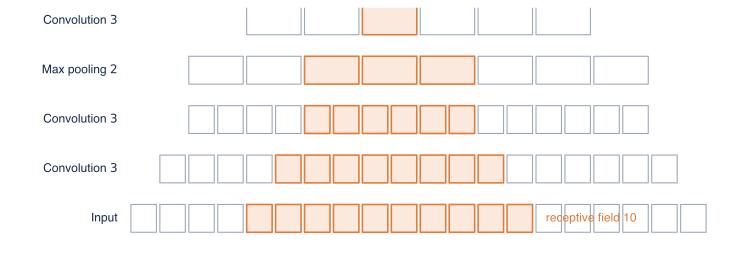
Figure 10.2 How the receptive field grows. A one-dimensional stack of layers, from the input (bottom) through two convolutions with kernel size 3, a max pooling with size 2 and stride 2, and another convolution (top). The highlighted squares in each row are the units that can affect the highlighted unit in the top row. The receptive field grows by 2 per convolution, by 1 for the pooling, and then by 4 for the next convolution, because after pooling each step covers two input positions (equation 10.5).

Two refinements keep this honest. The receptive field is the region that can affect a unit; in a trained network the influence is concentrated near its center and falls off towards the edges, so the effective receptive field is smaller [11]. And stacking small kernels is more economical than using large ones: two $3 \times 3$ layers have the same $5 \times 5$ receptive field as one $5 \times 5$ layer but use $2 \times 9 = 18$ rather than 25 weights per pair of channels, and add a second nonlinearity. This argument made $3 \times 3$ kernels standard [7].

Pooling and strided convolution

Max pooling with size 2 and stride 2 divides each channel into $2 \times 2$ blocks and keeps the largest value in each, halving the height and width and quartering the number of values. For the block

$$\begin{bmatrix} 1 & 3 & 2 & 0 \\ 4 & 2 & 1 & 1 \\ 0 & 1 & 5 & 2 \\ 2 & 2 & 3 & 4 \end{bmatrix} \ \xrightarrow{\ \text{max}\ }\ \begin{bmatrix} 4 & 2 \\ 2 & 5 \end{bmatrix}, \qquad \xrightarrow{\ \text{average}\ }\ \begin{bmatrix} 2.5 & 1 \\ 1.25 & 3.5 \end{bmatrix}$$

Average pooling keeps the mean instead. Pooling has no parameters. Its maximum makes the output unchanged when a feature moves within its block, a small amount of invariance to shifts. A strided convolution, a convolution with $S = 2$, downsamples while learning how to combine the values, and many modern networks use it instead of pooling. At the end of a classifier, global average pooling averages each channel over all positions, turning a $C \times H \times W$ array into a vector of $C$ numbers that no longer depends on where anything is.

Tasks that need an output per pixel, such as the segmentation of article 1, must grow the feature maps back to the input size. Transposed convolutions do this with learned weights; they are the transpose of the matrix of a strided convolution, just as the backward pass of section 3 was. Encoder–decoder networks such as U-Net [12] downsample to gather context, upsample back, and add skip connections that carry fine detail from the early layers to the late ones.

6. A complete classifier

We now assemble a small network for $32 \times 32$ color images in 10 classes, the size of the CIFAR-10 benchmark. It has three stages. Each stage has two $3 \times 3$ convolutions with padding 1, each followed by ReLU, and then a $2 \times 2$ max pooling; each stage doubles the number of channels while the pooling halves the height and width. Global average pooling and one fully connected layer produce the 10 scores:

Layer	Output shape	Parameters	Multiply-adds	Receptive field
Input	$3 \times 32 \times 32$			1
Conv $3 \times 3$, 3 → 32	$32 \times 32 \times 32$	896	884,736	3
Conv $3 \times 3$, 32 → 32	$32 \times 32 \times 32$	9,248	9,437,184	5
Max pool $2 \times 2$	$32 \times 16 \times 16$	0		6
Conv $3 \times 3$, 32 → 64	$64 \times 16 \times 16$	18,496	4,718,592	10
Conv $3 \times 3$, 64 → 64	$64 \times 16 \times 16$	36,928	9,437,184	14
Max pool $2 \times 2$	$64 \times 8 \times 8$	0		16
Conv $3 \times 3$, 64 → 128	$128 \times 8 \times 8$	73,856	4,718,592	24
Conv $3 \times 3$, 128 → 128	$128 \times 8 \times 8$	147,584	9,437,184	32
Max pool $2 \times 2$	$128 \times 4 \times 4$	0		36
Global average pool	128	0		whole image
Fully connected, 128 → 10	10	1,290	1,280	whole image
Total		288,298	38,634,752

The table shows the typical shape of a convolutional network. The spatial size shrinks from $32 \times 32$ to $4 \times 4$ while the number of channels grows from 3 to 128: the network trades where for what. The parameters concentrate in the late layers, which have many channels, while the computation is spread evenly, because each stage halves the area and doubles the channels. By the last convolution the receptive field, 32, spans the whole image. The whole network has 288,298 parameters. A fully connected layer from the 3,072 input values would reach that number with only 94 hidden units, before any further layers.

Real networks follow the same pattern at larger scale. LeNet-5 [3], from 1998, read handwritten digits with about 60,000 parameters. AlexNet [4], whose victory in the 2012 ImageNet competition started the deep learning era in computer vision, had about 60 million parameters, most in its final fully connected layers. VGG-16 [7] had about 138 million parameters built from stacked $3 \times 3$ convolutions. Article 11 describes the residual networks [6] that followed, which are deeper but, thanks to global average pooling and $1 \times 1$ convolutions, much smaller.

7. Learning a filter

The kernels of a convolutional network are parameters like any others, trained by gradient descent on the loss. A small experiment shows a kernel being learned and also shows why this can be slow.

We take the grayscale cat photograph of article 2, with pixel values between 0 and 1, and ask a single convolutional layer, one $3 \times 3$ kernel and a bias, to reproduce the output of the Sobel kernel $K_x$ at every position. The training data are the 133,802 positions where the kernel fits inside the image, and the loss is the mean squared error between the layer's output and the Sobel output. This is a toy: a real network is trained on labels, not on the output of a known filter. But it isolates the learning of one kernel. We start from random weights and run full-batch gradient descent with the largest stable learning rate.

Figure 10.3 shows the result. The kernel does converge to the Sobel kernel exactly, but slowly: after 100 steps it still looks random, after 1,000 a left–right structure has appeared, after 10,000 the loss is 0.00016 and the kernel is close, and after 100,000 steps the weights match $K_x$ to two decimal places.

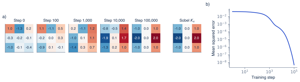
Figure 10.3 A convolution kernel learning to become the Sobel filter. A single $3 \times 3$ kernel with a bias is trained by gradient descent to reproduce the Sobel output $K_x$ on the grayscale cat photograph of article 2. a) The kernel at the start and after 100, 1,000, 10,000 and 100,000 steps, next to the Sobel kernel; red is positive, blue negative. b) The mean squared error during training. The kernel reaches the Sobel weights exactly, but it takes tens of thousands of steps.

The slowness has the same cause as the analysis of early stopping in article 9. The loss is quadratic in the ten parameters, and its curvature differs enormously between directions: the largest eigenvalue of its matrix of second derivatives is 5.99 and the smallest is 0.00026, a ratio of 23,000. The direction of high curvature is the kernel's overall sum, which multiplies the average brightness of each patch. The directions of low curvature are the differences between neighbouring weights, which multiply differences between neighbouring pixels, and in natural images neighbouring pixels are nearly equal. A learning rate small enough to be stable in the steep direction makes progress in the flat directions about 23,000 times slower. Unfortunately, the flat directions are exactly the ones that detect edges. Subtracting the mean brightness from the image reduces the ratio to about 7,700 but does not remove the problem, because it comes from the correlations between neighbouring pixels, not from their mean.

This is one reason why practical training uses adaptive optimizers such as Adam, which rescale each direction separately, and normalization layers (article 11), which keep the inputs of every layer centered and scaled. It also explains an observation about trained networks: kernels in the first layer of large image classifiers tend to look like oriented edge detectors and color blobs [4], [9]. Edges are what distinguishes images from one another once their overall brightness is accounted for, and a network trained long enough with a good optimizer finds them.

8. What convolutional networks learn, and where they fall short

Visualizations of trained networks [9], [10] show a progression with depth. Early layers respond to edges and color contrasts, middle layers to textures and simple shapes, and late layers to object parts such as eyes, wheels or text, and to whole objects. This hierarchy was not specified by anyone; it emerged from training on labels, and it is the learned counterpart of the hand-designed pipelines of article 2. It is an empirical description of what typical networks learn, not a guarantee.

Three limitations are worth knowing.

Shift invariance is only approximate. Convolution is equivariant to shifts, but strides and pooling sample the feature maps on a coarse grid, and a shift of one pixel can move a feature across a block boundary. Trained classifiers can change their prediction when an image is shifted by a single pixel [13]. Blurring before downsampling, as in classical signal processing, reduces the effect [14].

Texture over shape. Networks trained on ImageNet rely more on texture than humans do: shown an image with the shape of a cat and the texture of elephant skin, they tend to answer "elephant" [15]. What a network learns depends on what in the training data predicts the labels, not on what a person would consider the defining feature.

Adversarial examples. Changes to an image too small for a person to notice, chosen by following the gradient of the loss with respect to the input (section 3 shows how to compute it), can change a network's prediction to almost any class [16]. This sensitivity is not specific to convolutional networks and is not fully understood.

9. Terminology

• A convolutional layer applies equation 10.4. Its kernels, also called filters, are its learned weights; each output channel has one.
• The output of one channel at every position is a feature map. The channels of an array are its first dimension; a color image has three.
• Padding, stride and dilation control where the kernel is applied (equation 10.2).
• The receptive field of a unit is the input region that can affect it (equation 10.5).
• Pooling layers (max, average, global average) summarize blocks of values without parameters. Downsampling reduces the height and width; upsampling, for example with a transposed convolution, increases them.
• A convolutional neural network (CNN) is a network built mainly from convolutional layers, usually ending in global pooling and fully connected layers for classification.

Summary

A convolutional layer is a fully connected layer restricted in two ways: each output depends only on a small neighbourhood of the input, and every position uses the same weights. The restriction reduces the parameters from millions to hundreds, builds in equivariance to shifts, and lets each kernel learn from every position of every image. Its gradients are themselves convolutions. With several input and output channels, each output channel is a learned detector applied across all input channels. Stacking layers widens the receptive field, and pooling or strided convolutions widen it faster while trading spatial resolution for more channels. A complete classifier follows this pattern and ends with global average pooling. The kernels are learned by gradient descent; on natural images this is slow for the edge-like directions because neighbouring pixels are strongly correlated, which is one motivation for adaptive optimizers and normalization. Trained networks learn a hierarchy from edges to objects, but their invariance to shifts is only approximate and they can rely on cues a person would not. Article 11 shows how to train such networks with hundreds of layers.

Notes

History. Fukushima's Neocognitron [2] (1980) stacked layers of local, shared feature detectors with downsampling, inspired by the visual cortex, but was not trained by gradient descent. LeCun and colleagues trained convolutional networks with backpropagation to read handwritten zip codes [5] and later digits on bank cheques [3]. The ImageNet result of Krizhevsky, Sutskever and Hinton [4] in 2012 combined a large convolutional network, ReLU activations, dropout, data augmentation and training on GPUs.

Convolution arithmetic. Dumoulin and Visin [8] illustrate how padding, stride, dilation and transposed convolutions interact, with diagrams for each case.

Other dimensions and data. One-dimensional convolutions process audio and other time series, and three-dimensional ones process video and medical volumes. Graphs, whose nodes have no fixed grid of neighbours, need a different generalization (graph neural networks). Transformers (article 12) remove locality altogether and let every position attend to every other; applied to images, they need large datasets or strong augmentation to compensate for the lost restriction.

Reading further. Chapter 10 of Understanding Deep Learning [1] covers convolutional networks for one- and two-dimensional data, including the invariance and equivariance arguments of section 1.

Problems

Problem 10.1 Apply the kernel $(-1, 0, 1)$ with zero padding to $\mathbf{x} = (2, 2, 2, 5, 5, 5)$. What does the output detect? (Answer: $(2, 0, 3, 3, 0, -5)$. Inside the signal it is nonzero only around the step from 2 to 5; the values at the two ends come from the zero padding.)

Problem 10.2 How many parameters does a $5 \times 5$ convolutional layer from 16 to 32 channels have? How many multiply-adds does it need on a $28 \times 28$ output? (Answer: $32 \times (16 \times 25 + 1) = 12{,}832$; $28 \times 28 \times 32 \times 16 \times 25 = 10{,}035{,}200$.)

Problem 10.3 Using equation 10.2, what is the output length for an input of length 32 with $K = 3$, $P = 1$, $S = 2$? (Answer: $\lfloor (32 + 2 - 2 - 1)/2 \rfloor + 1 = 16$.)

Problem 10.4 Compute the receptive field of four $3 \times 3$ convolutions with stride 1, and of the sequence conv 3, conv 3 with stride 2, conv 3, conv 3. (Answer: 9; for the second, $r = 3, 5, 9, 13$, because after the strided layer each step covers two pixels.)

Problem 10.5 For the input $\mathbf{x} = (0, 1, 3, 2, 0, 0)$ and the error signal $\boldsymbol{\delta} = (1, 0, 0, 0, 0, 0)$, compute the gradients of the three kernel weights with equation 10.3. (Answer: $\partial\ell/\partial\omega_1 = x_0 = 0$, $\partial\ell/\partial\omega_2 = x_1 = 0$, $\partial\ell/\partial\omega_3 = x_2 = 1$.)

Problem 10.6 Show that a layer applying equation 10.1 to every position is equivariant to circular shifts when the padding wraps around (so that $x_0 = x_6$ and $x_7 = x_1$). (Hint: write the shifted input as $x'_i = x_{i-1}$ with indices taken modulo 6, and substitute into equation 10.1.)

References

• 1: Simon J.D. Prince (2023). Understanding Deep Learning. MIT Press.
• 2: Kunihiko Fukushima (1980). Neocognitron: a self-organizing neural network model for a mechanism of pattern recognition unaffected by shift in position. Biological Cybernetics 36(4), 193–202.
• 3: Yann LeCun, Léon Bottou, Yoshua Bengio and Patrick Haffner (1998). Gradient-based learning applied to document recognition. Proceedings of the IEEE 86(11), 2278–2324.
• 4: Alex Krizhevsky, Ilya Sutskever and Geoffrey Hinton (2012). ImageNet classification with deep convolutional neural networks. Advances in Neural Information Processing Systems 25.
• 5: Yann LeCun, Bernhard Boser, John Denker, Donnie Henderson, Richard Howard, Wayne Hubbard and Lawrence Jackel (1989). Backpropagation applied to handwritten zip code recognition. Neural Computation 1(4), 541–551.
• 6: Kaiming He, Xiangyu Zhang, Shaoqing Ren and Jian Sun (2016). Deep residual learning for image recognition. IEEE Conference on Computer Vision and Pattern Recognition.
• 7: Karen Simonyan and Andrew Zisserman (2015). Very deep convolutional networks for large-scale image recognition. International Conference on Learning Representations.
• 8: Vincent Dumoulin and Francesco Visin (2016). A guide to convolution arithmetic for deep learning. arXiv:1603.07285.
• 9: Matthew Zeiler and Rob Fergus (2014). Visualizing and understanding convolutional networks. European Conference on Computer Vision.
• 10: Chris Olah, Alexander Mordvintsev and Ludwig Schubert (2017). Feature visualization. Distill.
• 11: Wenjie Luo, Yujia Li, Raquel Urtasun and Richard Zemel (2016). Understanding the effective receptive field in deep convolutional neural networks. Advances in Neural Information Processing Systems 29.
• 12: Olaf Ronneberger, Philipp Fischer and Thomas Brox (2015). U-Net: convolutional networks for biomedical image segmentation. Medical Image Computing and Computer-Assisted Intervention.
• 13: Aharon Azulay and Yair Weiss (2019). Why do deep convolutional networks generalize so poorly to small image transformations? Journal of Machine Learning Research 20(184), 1–25.
• 14: Richard Zhang (2019). Making convolutional networks shift-invariant again. International Conference on Machine Learning.
• 15: Robert Geirhos, Patricia Rubisch, Claudio Michaelis, Matthias Bethge, Felix Wichmann and Wieland Brendel (2019). ImageNet-trained CNNs are biased towards texture; increasing shape bias improves accuracy and robustness. International Conference on Learning Representations.
• 16: Christian Szegedy, Wojciech Zaremba, Ilya Sutskever, Joan Bruna, Dumitru Erhan, Ian Goodfellow and Rob Fergus (2014). Intriguing properties of neural networks. International Conference on Learning Representations.