Residual networks and normalization: training very deep networks

Article 7 showed that depth can make a network far more expressive, and article 8 derived the initialization that keeps signals the right size at the start of training. Yet in 2015 the deepest networks that trained well had about twenty layers. Adding more layers to a plain convolutional network made it worse, even on its training data. This article explains why, and introduces the two ideas that removed the limit: residual connections, which add each layer's output to its input, and normalization layers, which rescale the activations inside the network. Together they made networks with a hundred layers routine, and they are part of almost every modern architecture, including the transformers of article 12. We derive what each does to the forward signal and to the gradients, verify the derivations by simulation, and separate what is proved about them from what is only observed.

1. Deeper is not automatically better

He and colleagues trained plain convolutional networks of 20 and 56 layers on the CIFAR-10 images [2]. The 56-layer network had higher error than the 20-layer one, on the test set and on the training set. Higher training error rules out overfitting (article 9) as the explanation. It is also not a matter of representation: the deeper network could imitate the shallower one by setting its extra layers to the identity, so its best possible training error is at most as low. The deeper network was harder to optimize. They called this the degradation problem.

Initialization alone does not cure it. He initialization (article 8) keeps the size of the activations and error signals constant on average, but deep products of random matrices still scramble the information the gradient carries. One way to see this is to look at how the gradient changes with the input. Figure 11.1 plots the derivative $\partial y / \partial x$ of three networks with one input and one output, as the input moves along a line. For a shallow network the derivative is a simple function of $x$: nearby inputs have similar gradients. For a plain network with 100 layers it looks like noise. Averaged over ten random networks, the correlation between the derivatives at neighbouring points of the line is 0.98 for the shallow network, and falls to 0.90, 0.70 and 0.50 for plain networks of 24, 50 and 100 layers. Balduzzi and colleagues called this the shattered gradients problem [9]. If the gradient at one input says little about the gradient at a nearby input, a gradient step computed on a batch of examples is a poor guide for the inputs nearby, and training makes slow progress.

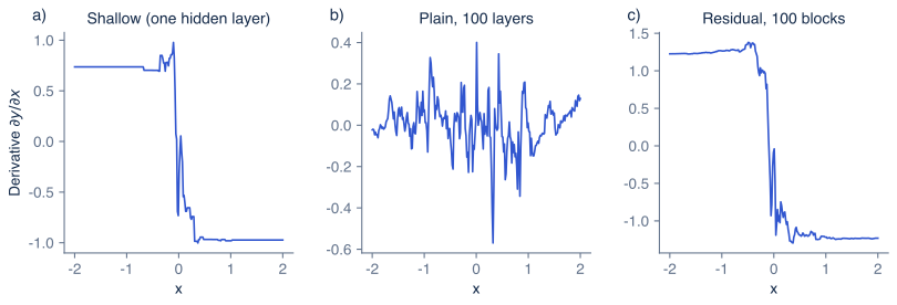
Figure 11.1 Shattered gradients. The derivative $\partial y / \partial x$ of three randomly initialized ReLU networks of width 100 with a scalar input and output, along 256 inputs between $-2$ and 2. a) A shallow network: the derivative changes smoothly with $x$. b) A plain network with 100 layers and He initialization: the derivative at one input is nearly unrelated to the derivative at its neighbours (correlation 0.50 between neighbouring points, averaged over ten networks). c) A residual network with 100 blocks (section 2): the structure of the shallow network survives (correlation 0.97).

The third panel of figure 11.1 shows the network that keeps the structure: a residual network with 100 blocks. We now introduce it.

2. Residual connections

A residual block computes a function $\mathbf{F}_k$ of its input, the residual branch, and adds the result to the input:

$$\mathbf{h}_{k+1} = \mathbf{h}_k + \mathbf{F}_k(\mathbf{h}_k) \tag{11.1}$$

The branch $\mathbf{F}_k$ is a small network, typically two layers with an activation function between them, and its output must have the same shape as its input so that the two can be added. The connection that carries $\mathbf{h}_k$ around the branch is the skip connection or shortcut. In words: each block computes a correction and adds it to what it received, rather than replacing it. If the branch outputs zero, the block is the identity; a deep network made of such blocks can therefore represent the shallower network obtained by deleting any of them, which is exactly the property the degradation problem seemed to lack.

Unravelling a residual network

Substituting one block into the next shows what a residual network computes. With three blocks and input $\mathbf{x}$:

$$\mathbf{y} = \mathbf{x} + \mathbf{F}_1(\mathbf{x}) + \mathbf{F}_2\big(\mathbf{x} + \mathbf{F}_1(\mathbf{x})\big) + \mathbf{F}_3\Big(\mathbf{x} + \mathbf{F}_1(\mathbf{x}) + \mathbf{F}_2\big(\mathbf{x} + \mathbf{F}_1(\mathbf{x})\big)\Big) \tag{11.2}$$

Each block can be either passed through or skipped, so there are $2^3 = 8$ paths from input to output, of lengths 0, 1, 2 and 3 blocks, with $1, 3, 3, 1$ paths of each length. A network with $K$ blocks has $2^K$ paths, and the number of paths through $k$ blocks is $\binom{K}{k}$: most paths have about half the network's depth. A plain network, by contrast, has a single path through every layer.

The gradient always has a direct path

The derivative of one block's output with respect to its input follows from equation 11.1:

$$\frac{\partial \mathbf{h}_{k+1}}{\partial \mathbf{h}_k} = \mathbf{I} + \frac{\partial \mathbf{F}_k}{\partial \mathbf{h}_k} \tag{11.3}$$

where $\mathbf{I}$ is the identity matrix, from the skip connection, and the second term is the Jacobian of the branch. Backpropagation through $K$ blocks multiplies these matrices (article 8, equation 8.12), and expanding the product gives

$$\prod_{k=1}^{K}\Big(\mathbf{I} + \frac{\partial \mathbf{F}_k}{\partial \mathbf{h}_k}\Big) = \mathbf{I} + \sum_{k} \frac{\partial \mathbf{F}_k}{\partial \mathbf{h}_k} + \sum_{k > j} \frac{\partial \mathbf{F}_k}{\partial \mathbf{h}_k}\frac{\partial \mathbf{F}_j}{\partial \mathbf{h}_j} + \cdots \tag{11.4}$$

with one term per path of equation 11.2 (the order of the matrix products follows the order of the blocks). The first term is the identity: the error signal at the output reaches every block directly, unchanged, whatever the branches do. In a plain network, by contrast, the only term is the product of all the layers' Jacobians.

Scalar numbers make the difference concrete. In a plain chain of 20 layers whose derivatives all equal 0.5, the product is $0.5^{20} \approx 9.5 \times 10^{-7}$; with 0.9 it is 0.12 and with 1.1 it is 6.7. Every factor must be very close to 1 for the product to stay usable. In a residual chain the factors are $1 + c_k$, where $c_k$ is the branch's derivative. With $c_k = 0.05$ for all 20 blocks the product is $1.05^{20} = 2.65$, and with $c_k = -0.05$ it is $0.95^{20} = 0.36$. The branches only need to be small, not precisely tuned. If they are initialized to be exactly zero, the network starts as the identity map between its first and last layers, which is trivially trainable, and training grows each branch from there.

3. The variance of a residual network

Equation 11.1 has a cost. Each block adds its branch's output to the signal, so the signal grows. At initialization, with the last weights of each branch drawn independently with mean zero, the branch output is uncorrelated with $\mathbf{h}_k$, and the variances add:

$$\mathrm{Var}(\mathbf{h}_{k+1}) = \mathrm{Var}(\mathbf{h}_k) + \mathrm{Var}\big(\mathbf{F}_k(\mathbf{h}_k)\big) \tag{11.5}$$

If the branch is initialized so that it preserves the size of its input, as He initialization does for each layer, then $\mathrm{Var}(\mathbf{F}_k(\mathbf{h}_k)) \approx \mathrm{Var}(\mathbf{h}_k)$ and the variance roughly doubles with every block: after 50 blocks it has grown by about $2^{50} \approx 10^{15}$. The residual network has traded the vanishing products of a plain network for an exploding sum.

Figure 11.2 checks this with a simulation of 50 blocks of width 100, each branch two ReLU layers with He initialization, on a batch of 256 random inputs. Without any correction (orange), the variance is 2.0 after one block, 1,490 after 10 and $8 \times 10^{15}$ after 50. Three remedies are in use, and the figure shows two of them:

• Scale the branches. Multiplying each branch by $1/\sqrt{K}$ makes it add only $1/K$ of the current variance, so $\mathrm{Var}(\mathbf{h}_K) \approx (1 + 1/K)^K\,\mathrm{Var}(\mathbf{x}) \le e\,\mathrm{Var}(\mathbf{x})$. The simulation gives 2.6 after 50 blocks (green).
• Initialize each branch to zero, by setting its last weights or the scale of its last normalization layer to zero [10]. The network then starts exactly at the identity, and the variance is constant at initialization.
• Normalize the branch's input. If each branch begins with a normalization layer (section 4), its input always has unit variance, so it adds a roughly constant amount of variance and the total grows only linearly with depth: 2.1 after one block and 48 after 50 (blue). Each new branch is then small relative to the signal it is added to, which biases the blocks towards the identity at initialization [11].

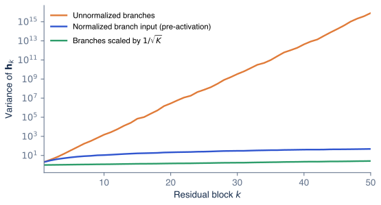
Figure 11.2 The variance of the signal through 50 residual blocks. Each block adds the output of a two-layer ReLU branch with He initialization (width 100, batch of 256 random inputs). Orange: unnormalized branches; the variance roughly doubles per block (equation 11.5). Blue: each branch starts with batch normalization, so it adds a roughly constant amount and the variance grows linearly. Green: each branch is multiplied by $1/\sqrt{50}$, and the variance grows only by a factor of about $e$. Note the logarithmic axis.

4. Batch normalization

Normalization layers rescale activations inside the network. The first and most influential is batch normalization [3]. It operates on each hidden unit (or, in a convolutional network, each channel) separately, using the values of that unit across the $B$ examples of the current batch. For one unit with pre-activations $z_1, \ldots, z_B$, it computes:

$$\mu = \frac{1}{B}\sum_{i=1}^{B} z_i, \qquad \sigma^2 = \frac{1}{B}\sum_{i=1}^{B} (z_i - \mu)^2, \qquad \hat{z}_i = \frac{z_i - \mu}{\sqrt{\sigma^2 + \epsilon}}, \qquad y_i = \gamma\,\hat{z}_i + \beta \tag{11.6}$$

We can break this down into three steps. First, compute the mean and variance of the unit over the batch. Second, subtract the mean and divide by the standard deviation, so that the normalized values $\hat{z}_i$ have mean 0 and variance 1 within the batch; the small constant $\epsilon$, such as $10^{-5}$, avoids division by zero. Third, scale and shift with two learned parameters per unit, $\gamma$ and $\beta$, so that the layer can still represent any mean and variance the network needs, including undoing the normalization. In a convolutional network, the mean and variance of a channel are taken over the batch and over all positions, so that every position is treated the same way.

For example, if one unit's pre-activations in a batch of four are $(2, 4, 6, 8)$, the mean is 5 and the variance is $(9 + 1 + 1 + 9)/4 = 5$. The normalized values are $(-1.342, -0.447, 0.447, 1.342)$, and with $\gamma = 2$ and $\beta = 1$ the outputs are $(-1.683, 0.106, 1.894, 3.683)$. In words: batch normalization makes every unit's values have a controlled mean and spread across the batch, whatever the layers before it did.

At prediction time there may be a single example, so the batch statistics are replaced by running averages of $\mu$ and $\sigma^2$ accumulated during training. The layer then becomes a fixed affine function, which can be merged into the preceding weights. Because $\beta$ plays the role of a bias, the layer before a batch normalization layer needs no bias of its own.

The backward pass

The batch statistics depend on every example in the batch, so each example's gradient depends on the others. Writing $g_i = \partial\ell/\partial\hat{z}_i = \gamma\,\partial\ell/\partial y_i$ and applying the chain rule through $\mu$ and $\sigma$ (with $\epsilon$ neglected) gives

$$\frac{\partial \ell}{\partial z_i} = \frac{1}{\sigma}\Big(g_i - \frac{1}{B}\sum_{j} g_j - \hat{z}_i\,\frac{1}{B}\sum_{j} g_j\,\hat{z}_j\Big) \tag{11.7}$$

In words: from the incoming gradient we remove its mean over the batch and its component along the normalized values, and divide by the standard deviation. Both removals have a reason. Adding a constant to every $z_i$ in the batch, or multiplying all of them by a positive number, leaves $\hat{z}$ unchanged, so the loss cannot depend on those two directions, and the gradient has no component along them. For $z = (2, 4, 6, 8)$ and $g = (1, 0, 0, 0)$, equation 11.7 gives $(0.134, -0.179, -0.045, 0.089)$, which sums to zero and is orthogonal to $\hat{z}$, and agrees with finite differences.

Why it helps

Batch normalization made networks train faster, at higher learning rates and with less careful initialization, and it was quickly adopted everywhere. Why it works is less settled than that it works. Four mechanisms are well supported:

• It controls the scale of the activations at every layer, during training as well as at initialization, which removes the variance growth of section 3 and much of the sensitivity to initialization.
• It makes each layer invariant to the scale of its weights. If the weights $\boldsymbol{\Omega}$ feeding a normalized unit are multiplied by $a > 0$, the pre-activations are multiplied by $a$ and equation 11.6 removes the factor: the output does not change. The gradient with respect to $a\boldsymbol{\Omega}$ is then $1/a$ times the gradient with respect to $\boldsymbol{\Omega}$, so a gradient step changes the weights' direction by an amount proportional to $1/\|\boldsymbol{\Omega}\|^2$. Large weights automatically get small effective learning rates, and weight decay, which shrinks the weights, raises the effective learning rate [12].
• It allows larger learning rates. Santurkar and colleagues [13] found that batch normalization makes the loss and its gradient change more smoothly as the parameters move, so larger steps remain stable.
• It adds noise. Each example is normalized with statistics that depend on the other examples in its batch, which acts as a mild regularizer (article 9).

The explanation in the original paper, that batch normalization reduces internal covariate shift (the change in each layer's input distribution as earlier layers train), is not well supported: Santurkar and colleagues deliberately injected distribution shift after normalization layers and training was unaffected [13].

Batch normalization also has costs. Its behaviour depends on the batch size: with small batches the statistics are noisy and accuracy suffers. Training and prediction compute different functions, a source of subtle bugs. And examples in a batch influence each other's outputs, which some tasks cannot allow.

5. Other normalizations

The alternatives differ in which values are normalized together. For a convolutional layer, the activations of a batch form an array of shape $B \times C \times H \times W$. Each method computes a mean and a variance over one group of these values and normalizes the group with them (figure 11.3):

Method	Statistics computed over	Depends on the batch?	Main use
Batch norm [3]	One channel, all examples and positions	Yes	Convolutional networks with large batches
Layer norm [5]	One example, all channels (and positions)	No	Transformers, recurrent networks
Group norm [6]	One example, a group of channels	No	Convolutional networks with small batches
Instance norm [7]	One example, one channel	No	Image style transfer

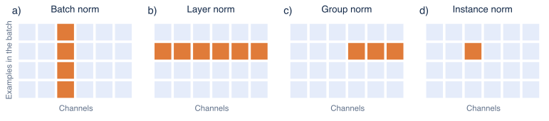
Figure 11.3 Which values each normalization uses. Each grid shows a batch of 4 examples (rows) with 6 channels (columns); each cell stands for all $H \times W$ positions of one channel of one example. The orange cells are normalized together, with one mean and one variance. a) Batch norm: one channel across the batch. b) Layer norm: all channels of one example. c) Group norm: a group of channels of one example. d) Instance norm: one channel of one example.

A small table shows the difference. Take a batch of four examples with three features each, one example per row:

$$\begin{bmatrix} 2 & 0 & 4 \\ 4 & 2 & 0 \\ 6 & 2 & 4 \\ 8 & 4 & 4 \end{bmatrix} \ \xrightarrow{\ \text{batch norm (columns)}\ }\ \begin{bmatrix} -1.342 & -1.414 & 0.577 \\ -0.447 & 0 & -1.732 \\ 0.447 & 0 & 0.577 \\ 1.342 & 1.414 & 0.577 \end{bmatrix}, \qquad \xrightarrow{\ \text{layer norm (rows)}\ }\ \begin{bmatrix} 0 & -1.225 & 1.225 \\ 1.225 & 0 & -1.225 \\ 1.225 & -1.225 & 0 \\ 1.414 & -0.707 & -0.707 \end{bmatrix}$$

Batch normalization makes each column have mean 0 and variance 1; each example's output depends on the other three examples. Layer normalization makes each row have mean 0 and variance 1; each example is normalized on its own, so it computes the same function at training and prediction time and works with any batch size, including one. That independence is why transformers, which often process one sequence at a time during generation, use layer normalization. RMSNorm [8] simplifies layer normalization further by dividing by the root mean square without subtracting the mean: the first row $(2, 0, 4)$ becomes $(0.775, 0, 1.549)$. It is cheaper and works about as well in large language models.

6. Residual block designs

The residual idea leaves open what goes inside the branch and where the normalization and activation go. Three designs cover most practice (figure 11.4).

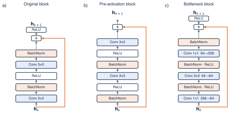
Figure 11.4 Three residual blocks. The orange line is the skip connection. a) The original block of He and colleagues [2]: two $3 \times 3$ convolutions, each followed by batch normalization, with a ReLU applied after the addition. b) The pre-activation block [4]: normalization and ReLU come before each convolution, and nothing is applied after the addition, so the skip connections form a clean identity path through the whole network. c) The bottleneck block used in deeper networks: $1 \times 1$ convolutions reduce 256 channels to 64 for the expensive $3 \times 3$ convolution and restore them afterwards.

Original and pre-activation blocks. In the original block (figure 11.4a), a ReLU follows the addition, so the signal passed to the next block is not exactly $\mathbf{h}_k + \mathbf{F}_k(\mathbf{h}_k)$. The pre-activation block (figure 11.4b) moves the normalization and activation inside the branch. Then $\mathbf{h}_K = \mathbf{h}_k + \sum_{j=k}^{K-1}\mathbf{F}_j(\mathbf{h}_j)$ holds exactly for any two blocks, and equation 11.4's identity term is untouched. He and colleagues found that this design trained networks of 1,000 layers better than the original [4]. Transformers use the same pattern with layer normalization (article 12).

Bottleneck blocks. A block of two $3 \times 3$ convolutions at 256 channels has $2 \times 9 \times 256 \times 256 = 1{,}179{,}648$ weights. The bottleneck block (figure 11.4c) applies the $3 \times 3$ convolution at 64 channels, between two $1 \times 1$ convolutions that reduce and restore the channel count, and has $256 \times 64 + 9 \times 64 \times 64 + 64 \times 256 = 69{,}632$ weights, 17 times fewer. ResNet-50, built from 16 such blocks, has about 25.6 million parameters, less than a fifth of VGG-16's, and was more accurate on ImageNet.

Changing the shape. Equation 11.1 needs the branch output to have the shape of its input. Where a network downsamples or changes the number of channels, the skip connection applies a $1 \times 1$ convolution with stride 2 (a projection shortcut) so that the shapes match.

Related designs. Highway networks [14] preceded residual networks with gated skip connections, whose gate is learned. DenseNets [15] concatenate the outputs of all earlier layers instead of adding them. The skip connections of U-Net (article 10) carry fine detail across the network rather than around a single block.

7. Why residual networks work

Three accounts are well supported; none is complete.

The identity path keeps gradients informative. This is the derivation of section 2, and it is exact: equation 11.4 contains a term that delivers the output's error signal to every block unchanged. Figure 11.1c shows the consequence for the shattering of section 1: with 100 blocks the correlation between neighbouring gradients is 0.97, almost that of a shallow network.

Residual networks behave like ensembles of shallower networks. Veit and colleagues [16] studied the paths of equation 11.2 empirically. Deleting a single block from a trained residual network barely changes its accuracy, while deleting a layer from a plain network like VGG destroys it, so no single path is essential. And in a residual network with 110 layers, most of the gradient during training came from paths only 10 to 34 layers deep. This suggests that residual networks avoid the difficulties of depth partly by not relying on their longest paths.

The loss surface is smoother. Li and colleagues [17] visualized loss surfaces along random directions in parameter space. Deep networks without skip connections had chaotic surfaces with many sharp local features, while the same networks with skip connections had smooth, nearly convex surfaces around the minimum found by training. Such visualizations are low-dimensional slices of a very high-dimensional surface, so they illustrate rather than prove.

8. Terminology

• A residual block computes $\mathbf{h} + \mathbf{F}(\mathbf{h})$. $\mathbf{F}$ is the residual branch, and the connection that bypasses it is the skip connection, shortcut or identity path. A network built from such blocks is a residual network (ResNet). The sequence of $\mathbf{h}_k$ is sometimes called the residual stream.
• A pre-activation block normalizes and activates before each weight layer inside the branch; a post-activation block does so after.
• A bottleneck block reduces the number of channels with a $1 \times 1$ convolution before an expensive layer and restores it afterwards. A projection shortcut is a skip connection with a $1 \times 1$ convolution that changes the shape.
• Batch, layer, group and instance normalization differ in the set of values they normalize together (figure 11.3). RMSNorm divides by the root mean square without subtracting the mean. The learned $\gamma$ and $\beta$ are the scale and shift (or gain and bias).

Summary

Plain networks with many layers train worse than shallow ones, even on their training data, because the gradient passes through a long product of layer Jacobians that scrambles it. Residual connections add each block's output to its input. The gradient then contains an identity term that reaches every block directly (equation 11.4), and the network behaves partly like an ensemble of shallower paths. The price is that variances add from block to block, doubling per block if nothing is done; scaling the branches, initializing them to zero or normalizing their inputs controls this. Batch normalization standardizes each unit over the batch and then rescales it with learned parameters; it keeps activations in range, makes each layer invariant to the scale of its weights, allows larger learning rates and adds a little regularizing noise, though the original explanation for its success is not supported. Layer normalization does the same per example and is the choice for transformers. With these tools, networks of a hundred layers or more train reliably. Article 12 combines residual connections and layer normalization with a new kind of layer, attention, to build the transformer.

Notes

Normalization-free networks. Careful initialization and scaling of the residual branches can replace normalization altogether. Fixup [10] initializes the last layer of every branch to zero and rescales the others, and trains residual networks with thousands of layers without normalization. Later work reached the accuracy of batch-normalized networks on ImageNet without any normalization layers, using scaled weight standardization and adaptive gradient clipping [18].

Weight normalization. Instead of normalizing activations, one can normalize the weights: write each weight vector as a length times a unit direction and learn the two separately. This gives the scale invariance of section 4 without depending on the batch [19].

Depth in practice. Residual connections make depth trainable, not free. Very deep residual networks are often less accurate than wider, shallower ones of the same cost, and the best depth is found by experiment. He and colleagues trained a 1,202-layer network on CIFAR-10; it fitted the training set but had higher test error than their 110-layer network, which they attributed to overfitting [2].

Reading further. Chapter 11 of Understanding Deep Learning [1] covers residual networks, the variance analysis of section 3, batch normalization and the shattered gradients of section 1.

Problems

Problem 11.1 Apply batch normalization (with $\gamma = 1$, $\beta = 0$, $\epsilon = 0$) to $(1, 3, 5, 7)$. Compare with the example of section 4 and explain the result. (Answer: the mean is 4 and the variance 5, so the output is again $(-1.342, -0.447, 0.447, 1.342)$; the input is the example's input minus 1, and batch normalization removes any shift.)

Problem 11.2 How many paths run through a residual network with 4 blocks? How many of them pass through exactly two blocks? (Answer: $2^4 = 16$; $\binom{4}{2} = 6$.)

Problem 11.3 Show that with $\epsilon = 0$, batch normalization gives the same output for $a z_i + c$ as for $z_i$, for any $a > 0$ and any $c$. (Hint: the mean becomes $a\mu + c$ and the standard deviation $a\sigma$.)

Problem 11.4 If each of 10 residual branches adds as much variance as its input has, by what factor does the variance grow? What if each branch is multiplied by $1/\sqrt{10}$? (Answer: $2^{10} = 1{,}024$; $1.1^{10} \approx 2.59$.)

Problem 11.5 Apply layer normalization (with $\gamma = 1$, $\beta = 0$, $\epsilon = 0$) to one example with features $(1, 2, 3, 6)$. (Answer: mean 3, variance 3.5, output $(-1.069, -0.535, 0, 1.604)$.)

Problem 11.6 How many weights does a bottleneck block with 512 outer channels and 128 inner channels have, ignoring biases and normalization parameters? (Answer: $512 \times 128 + 9 \times 128 \times 128 + 128 \times 512 = 278{,}528$.)

Problem 11.7 In a scalar residual chain of 100 blocks whose branch derivatives all equal $c$, compute the product of equation 11.4 for $c = 0.01$ and $c = -0.01$. (Answer: $1.01^{100} \approx 2.70$ and $0.99^{100} \approx 0.366$.)

References

• 1: Simon J.D. Prince (2023). Understanding Deep Learning. MIT Press.
• 2: Kaiming He, Xiangyu Zhang, Shaoqing Ren and Jian Sun (2016). Deep residual learning for image recognition. IEEE Conference on Computer Vision and Pattern Recognition.
• 3: Sergey Ioffe and Christian Szegedy (2015). Batch normalization: accelerating deep network training by reducing internal covariate shift. International Conference on Machine Learning.
• 4: Kaiming He, Xiangyu Zhang, Shaoqing Ren and Jian Sun (2016). Identity mappings in deep residual networks. European Conference on Computer Vision.
• 5: Jimmy Lei Ba, Jamie Ryan Kiros and Geoffrey Hinton (2016). Layer normalization. arXiv:1607.06450.
• 6: Yuxin Wu and Kaiming He (2018). Group normalization. European Conference on Computer Vision.
• 7: Dmitry Ulyanov, Andrea Vedaldi and Victor Lempitsky (2016). Instance normalization: the missing ingredient for fast stylization. arXiv:1607.08022.
• 8: Biao Zhang and Rico Sennrich (2019). Root mean square layer normalization. Advances in Neural Information Processing Systems 32.
• 9: David Balduzzi, Marcus Frean, Lennox Leary, J.P. Lewis, Kurt Wan-Duo Ma and Brian McWilliams (2017). The shattered gradients problem: if resnets are the answer, then what is the question? International Conference on Machine Learning.
• 10: Hongyi Zhang, Yann Dauphin and Tengyu Ma (2019). Fixup initialization: residual learning without normalization. International Conference on Learning Representations.
• 11: Soham De and Samuel Smith (2020). Batch normalization biases residual blocks towards the identity function in deep networks. Advances in Neural Information Processing Systems 33.
• 12: Twan van Laarhoven (2017). L2 regularization versus batch and weight normalization. arXiv:1706.05350.
• 13: Shibani Santurkar, Dimitris Tsipras, Andrew Ilyas and Aleksander Mądry (2018). How does batch normalization help optimization? Advances in Neural Information Processing Systems 31.
• 14: Rupesh Kumar Srivastava, Klaus Greff and Jürgen Schmidhuber (2015). Training very deep networks. Advances in Neural Information Processing Systems 28.
• 15: Gao Huang, Zhuang Liu, Laurens van der Maaten and Kilian Weinberger (2017). Densely connected convolutional networks. IEEE Conference on Computer Vision and Pattern Recognition.
• 16: Andreas Veit, Michael Wilber and Serge Belongie (2016). Residual networks behave like ensembles of relatively shallow networks. Advances in Neural Information Processing Systems 29.
• 17: Hao Li, Zheng Xu, Gavin Taylor, Christoph Studer and Tom Goldstein (2018). Visualizing the loss landscape of neural nets. Advances in Neural Information Processing Systems 31.
• 18: Andrew Brock, Soham De, Samuel Smith and Karen Simonyan (2021). High-performance large-scale image recognition without normalization. International Conference on Machine Learning.
• 19: Tim Salimans and Diederik Kingma (2016). Weight normalization: a simple reparameterization to accelerate training of deep neural networks. Advances in Neural Information Processing Systems 29.