Transformers: attention over a sequence

Convolutional networks (article 10) suit images because nearby pixels matter most and a pattern means the same thing everywhere. Text breaks both assumptions. In "The cat that the dog chased all morning finally fell asleep", whether the verb "fell" refers to the cat or the dog depends on words seven positions earlier, and which earlier word matters depends on the content, not on a fixed offset. Texts also vary in length, from a few words to whole books. A fully connected network needs a fixed input size, and a convolution looks only at a fixed neighbourhood with weights tied to relative position. This article introduces the layer that handles all three requirements, self-attention, in which every position computes a weighted average of all positions, with weights computed from their content. We work through self-attention with three tokens and actual numbers, write it in matrix form and derive its properties, explain the scaling, the position information and the multiple heads it needs in practice, and assemble the transformer: self-attention combined with the residual connections and layer normalization of article 11. We then count the parameters of a real model, GPT-2, and describe how transformers are trained to model language.

1. Text as a sequence of vectors

A transformer does not read characters. Text is first split into tokens, units from a fixed vocabulary of typically 30,000 to 100,000 entries. Common words are single tokens; rare words are split into pieces that do occur often, such as "un", "believ" and "able". This subword tokenization [4] lets a finite vocabulary represent any string while keeping frequent words whole. Each token is then replaced by a learned vector of $D$ numbers, its embedding. With a vocabulary of $|\mathcal{V}|$ tokens, the embeddings form a matrix $\boldsymbol{\Omega}_e \in \mathbb{R}^{D \times |\mathcal{V}|}$, and token number $t$ is mapped to column $t$. For GPT-2 [6], with $|\mathcal{V}| = 50{,}257$ and $D = 768$, the embedding matrix alone has 38,597,376 parameters. The embeddings are trained with the rest of the network.

A text of $N$ tokens thus becomes $N$ vectors $\mathbf{x}_1, \ldots, \mathbf{x}_N$, each of size $D$. We collect them as the columns of a matrix $\mathbf{X} \in \mathbb{R}^{D \times N}$, one column per token, matching the convention of articles 7 and 8. A layer for this data should:

1. accept any number $N$ of columns, with the same parameters;
2. treat every position by the same rule, as a convolution does; and
3. let each position draw information from any other position, with the choice of which positions depending on their content.

2. Self-attention: a worked example

Self-attention computes, for every position $n$, a new vector that is a weighted average of vectors derived from all positions. We start with three tokens of dimension 2 and actual numbers. We defer the general matrix form until section 3, and for now leave out the biases.

The three input vectors are the columns of

$$\mathbf{X} = \begin{bmatrix} 1 & 0 & 1 \\ 0 & 1 & 1 \end{bmatrix}$$

so $\mathbf{x}_1 = (1, 0)$, $\mathbf{x}_2 = (0, 1)$ and $\mathbf{x}_3 = (1, 1)$. Self-attention applies three different linear maps to every token. The query $\mathbf{q}_n = \boldsymbol{\Omega}_q \mathbf{x}_n$ describes what position $n$ is looking for. The key $\mathbf{k}_m = \boldsymbol{\Omega}_k \mathbf{x}_m$ describes what position $m$ offers. The value $\mathbf{v}_m = \boldsymbol{\Omega}_v \mathbf{x}_m$ is what position $m$ contributes if it is chosen. We take

$$\boldsymbol{\Omega}_q = \begin{bmatrix} 1 & 0 \\ 1 & 2 \end{bmatrix}, \qquad \boldsymbol{\Omega}_k = \begin{bmatrix} 1 & 1 \\ 0 & 1 \end{bmatrix}, \qquad \boldsymbol{\Omega}_v = \begin{bmatrix} 1 & 0 \\ 0 & 1 \end{bmatrix}$$

The value matrix is the identity only to keep the arithmetic short: each value equals its input. The queries are $\mathbf{q}_1 = (1, 1)$, $\mathbf{q}_2 = (0, 2)$, $\mathbf{q}_3 = (1, 3)$, and the keys are $\mathbf{k}_1 = (1, 0)$, $\mathbf{k}_2 = (1, 1)$, $\mathbf{k}_3 = (2, 1)$.

The layer computes three things, in order:

$$s_{mn} = \mathbf{k}_m^\top \mathbf{q}_n, \qquad a_{mn} = \frac{\exp(s_{mn})}{\sum_{m'=1}^{N} \exp(s_{m'n})}, \qquad \mathbf{sa}_n = \sum_{m=1}^{N} a_{mn}\, \mathbf{v}_m \tag{12.1}$$

First, a score $s_{mn}$ for every pair: the dot product of position $m$'s key with position $n$'s query, large when the two point in similar directions. Second, for each query $n$, a softmax over all keys $m$ (article 4) turns the scores into attention weights $a_{mn}$, which are positive and sum to 1 over $m$. Third, the output for position $n$ is the average of all the values, weighted by those weights. In words: each position asks a question, compares it with what every position offers, and takes a mixture of their contributions in proportion to how well they match.

For our numbers, the scores, with keys as rows and queries as columns, are

$$\mathbf{S} = \begin{bmatrix} 1 & 0 & 1 \\ 2 & 2 & 4 \\ 3 & 2 & 5 \end{bmatrix}$$

For the first query, the softmax of $(1, 2, 3)$ gives weights $(0.090, 0.245, 0.665)$: position 1 attends mostly to position 3. The second query's scores $(0, 2, 2)$ give $(0.063, 0.468, 0.468)$, split equally between positions 2 and 3. The third gives $(0.013, 0.265, 0.721)$. The outputs are the weighted averages of the values: for position 1, $0.090\,(1, 0) + 0.245\,(0, 1) + 0.665\,(1, 1) = (0.755, 0.910)$; for positions 2 and 3, $(0.532, 0.937)$ and $(0.735, 0.987)$. Figure 12.1a–b shows the scores and weights.

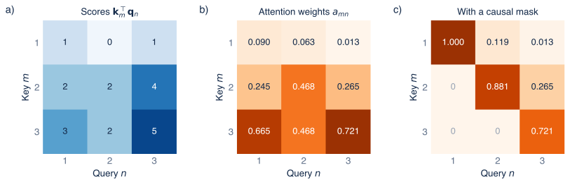
Figure 12.1 Self-attention with three tokens. Rows are keys $m$, columns are queries $n$. a) The scores $s_{mn} = \mathbf{k}_m^\top\mathbf{q}_n$ for the example of section 2. b) The attention weights: a softmax down each column, so each column sums to 1. Every position attends most to position 3, whose key is largest. c) The weights with the causal mask of section 8: each query may attend only to its own and earlier positions, so position 1 attends only to itself.

Three observations follow from the example. The score matrix is not symmetric: how much position 1 attends to position 3 ($a_{31}$) differs from how much 3 attends to 1 ($a_{13}$), because queries and keys use different maps. The weights are computed from the input, so the layer is not linear in $\mathbf{X}$ even though each value is: change $\mathbf{x}_3$ and both the values and the weights that mix them change. And nothing in equation 12.1 depends on $N$: a fourth token would add a row and a column to $\mathbf{S}$ and use the same three matrices.

3. Self-attention in matrix form

We now write the general layer, with biases, for $N$ tokens of dimension $D$. The queries, keys and values of all positions are the columns of three matrices:

$$\mathbf{Q} = \boldsymbol{\beta}_q \mathbf{1}^\top + \boldsymbol{\Omega}_q \mathbf{X}, \qquad \mathbf{K} = \boldsymbol{\beta}_k \mathbf{1}^\top + \boldsymbol{\Omega}_k \mathbf{X}, \qquad \mathbf{V} = \boldsymbol{\beta}_v \mathbf{1}^\top + \boldsymbol{\Omega}_v \mathbf{X} \tag{12.2}$$

where $\boldsymbol{\Omega}_q, \boldsymbol{\Omega}_k \in \mathbb{R}^{D_q \times D}$, $\boldsymbol{\Omega}_v \in \mathbb{R}^{D \times D}$ and $\mathbf{1}$ is a vector of $N$ ones, as in equation 7.8. All scores at once are the matrix $\mathbf{K}^\top\mathbf{Q} \in \mathbb{R}^{N \times N}$, whose entry in row $m$ and column $n$ is $\mathbf{k}_m^\top\mathbf{q}_n$. Applying the softmax to each column and mixing the values gives the whole layer:

$$\mathrm{Sa}(\mathbf{X}) = \mathbf{V}\, \mathrm{Softmax}\big(\mathbf{K}^\top \mathbf{Q}\big) \tag{12.3}$$

The shapes check: $(D \times N)$ times $(N \times N)$ gives $D \times N$, one output column per position. Column $n$ of the product is $\sum_m a_{mn}\mathbf{v}_m$, which is equation 12.1. Libraries usually store tokens as rows and write the same computation transposed, $\mathrm{softmax}(\mathbf{Q}\mathbf{K}^\top)\mathbf{V}$.

Parameters. The layer has $2D_q D + D^2$ weights and $2D_q + D$ biases, independent of $N$. With $D_q = D$, that is $3D^2 + 3D$.

Permutation equivariance. Reordering the tokens reorders the outputs in the same way. If $\mathbf{P}$ is a permutation matrix, replacing $\mathbf{X}$ by $\mathbf{X}\mathbf{P}$ replaces $\mathbf{Q}$, $\mathbf{K}$ and $\mathbf{V}$ by $\mathbf{Q}\mathbf{P}$, $\mathbf{K}\mathbf{P}$ and $\mathbf{V}\mathbf{P}$ (the bias terms are the same in every column). The scores become $\mathbf{P}^\top\mathbf{K}^\top\mathbf{Q}\mathbf{P}$: rows and columns permuted alike. A softmax down each column commutes with permuting rows within the column and with reordering the columns, so $\mathrm{Softmax}(\mathbf{P}^\top\mathbf{K}^\top\mathbf{Q}\mathbf{P}) = \mathbf{P}^\top\mathrm{Softmax}(\mathbf{K}^\top\mathbf{Q})\mathbf{P}$, and the output is $\mathbf{V}\mathbf{P}\mathbf{P}^\top\mathrm{Softmax}(\mathbf{K}^\top\mathbf{Q})\mathbf{P} = \mathrm{Sa}(\mathbf{X})\,\mathbf{P}$, because $\mathbf{P}\mathbf{P}^\top = \mathbf{I}$. The layer treats its input as a set: it has no idea which token came first. Section 5 adds that information back.

Cost. Computing $\mathbf{Q}$, $\mathbf{K}$ and $\mathbf{V}$ costs about $3ND^2$ multiply-adds, like a fully connected layer applied to each token. The scores cost $N^2 D_q$, and mixing the values another $N^2 D$. The attention matrix has $N^2$ entries, and memory and computation grow with the square of the sequence length: doubling the length of the text quadruples the attention cost. For short sequences the $ND^2$ terms dominate; for long ones the $N^2$ terms do.

4. Scaling the scores

Equation 12.3 has a problem when $D_q$ is large. Suppose the elements of a query and a key are independent with mean 0 and variance 1, roughly what initialization and normalization produce. Then the score $\mathbf{k}^\top\mathbf{q} = \sum_{i=1}^{D_q} k_i q_i$ is a sum of $D_q$ independent terms, each with mean 0 and variance $\mathbb{E}[k_i^2]\,\mathbb{E}[q_i^2] = 1$, so

$$\mathrm{Var}\big(\mathbf{k}^\top\mathbf{q}\big) = D_q \tag{12.4}$$

With $D_q = 64$, typical scores differ by around 8, and the softmax of numbers spread that widely puts nearly all the weight on the largest. A saturated softmax is a problem for training, not just for expressiveness. Its derivative is $\partial a_m / \partial s_{m'} = a_m(\mathbb{1}[m = m'] - a_{m'})$, which is close to zero for every entry when one weight is near 1 and the rest near 0, so almost no gradient flows back to the queries and keys.

The fix is to divide the scores by $\sqrt{D_q}$, which restores unit variance:

$$\mathrm{Sa}(\mathbf{X}) = \mathbf{V}\, \mathrm{Softmax}\Big(\frac{\mathbf{K}^\top \mathbf{Q}}{\sqrt{D_q}}\Big) \tag{12.5}$$

This is scaled dot-product attention [2]. Figure 12.2 shows the effect for 16 keys and random unit-variance vectors. Without scaling, the largest attention weight averages 0.21 for $D_q = 1$, 0.69 for $D_q = 16$, 0.92 for $D_q = 256$ and 0.96 for $D_q = 1024$: attention becomes a hard choice of one key. With scaling it stays between 0.21 and 0.25 for every $D_q$. In the worked example of section 2, $D_q = 2$ and scaling would have softened the second column from $(0.063, 0.468, 0.468)$ to $(0.108, 0.446, 0.446)$.

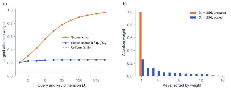
Figure 12.2 Why the scores are divided by $\sqrt{D_q}$. One query and 16 keys with independent standard normal elements. a) The largest of the 16 attention weights, averaged over 2,000 draws, as the dimension $D_q$ grows. Unscaled scores have variance $D_q$ (equation 12.4), so the softmax concentrates on one key; scaled scores keep the weights spread out. The dashed line is the uniform weight 1/16. b) One draw with $D_q = 256$: the 16 weights sorted from largest to smallest, unscaled (orange) and scaled (blue).

5. Positions

Because self-attention is permutation equivariant, "the dog chased the cat" and "the cat chased the dog" would produce the same outputs, merely reordered. Position information must be added explicitly. Three approaches are common.

Absolute sinusoidal encodings. The original transformer [2] added to each token's embedding a fixed vector that depends only on its position $p$, with elements

$$\mathrm{PE}_{p,\,2i} = \sin\big(p / 10000^{2i/D}\big), \qquad \mathrm{PE}_{p,\,2i+1} = \cos\big(p / 10000^{2i/D}\big) \tag{12.6}$$

for $i = 0, \ldots, D/2 - 1$. Each pair of elements is a sine and cosine at its own frequency, from one cycle every $2\pi$ positions for $i = 0$ down to very slow ones. For $D = 4$ and position 1, the encoding is $(\sin 1, \cos 1, \sin 0.01, \cos 0.01) = (0.841, 0.540, 0.010, 1.000)$. The fast pairs distinguish neighbouring positions, the slow ones distant positions, like the hands of a clock.

Learned absolute embeddings. GPT-2 instead learns a separate vector for each position up to a maximum length, a second embedding matrix of size $D \times 1024$ (786,432 parameters). It is simple and works well, but it cannot represent positions beyond the maximum seen in training.

Relative position through rotation. What usually matters is how far apart two tokens are, not where they are absolutely. Rotary position embedding (RoPE) [7] achieves this by rotating each query and key according to its position. In two dimensions, let $\mathbf{R}(\theta)$ be the rotation by angle $\theta$, and rotate the query at position $n$ by $n\theta$ and the key at position $m$ by $m\theta$. Rotations satisfy $\mathbf{R}(\alpha)^\top\mathbf{R}(\beta) = \mathbf{R}(\beta - \alpha)$, so the score is

$$\big(\mathbf{R}(m\theta)\,\mathbf{k}_m\big)^\top \big(\mathbf{R}(n\theta)\,\mathbf{q}_n\big) = \mathbf{k}_m^\top\, \mathbf{R}\big((n - m)\theta\big)\, \mathbf{q}_n \tag{12.7}$$

which depends on the positions only through their difference $n - m$. In $D_q$ dimensions, the elements are paired and each pair is rotated at its own frequency, as in equation 12.6. RoPE adds no parameters, and it is used in many recent language models.

6. Multi-head attention

One self-attention layer produces one set of weights per query: one way of deciding which positions are relevant. Language needs several at once: a verb may need its subject, its object and the tense marker elsewhere in the sentence. Multi-head attention runs $H$ self-attention layers, the heads, in parallel, each with its own queries, keys and values of size $D/H$, and combines their outputs:

$$\mathrm{MhSa}(\mathbf{X}) = \boldsymbol{\Omega}_c \begin{bmatrix} \mathrm{Sa}_1(\mathbf{X}) \\ \vdots \\ \mathrm{Sa}_H(\mathbf{X}) \end{bmatrix} + \boldsymbol{\beta}_c\mathbf{1}^\top \tag{12.8}$$

The $H$ outputs, each of shape $(D/H) \times N$, are stacked into a $D \times N$ matrix, and the output projection $\boldsymbol{\Omega}_c \in \mathbb{R}^{D \times D}$ mixes the heads. In words: every head attends in its own way, and the projection combines what they found. Splitting $D$ among the heads keeps the cost the same as one head of full size. The layer has $4D^2 + 4D$ parameters: $3D^2 + 3D$ for all the heads' queries, keys and values together, and $D^2 + D$ for the output projection. For $D = 768$ that is 2,362,368. GPT-2 small uses 12 heads of size 64.

7. The transformer layer

A transformer layer combines multi-head self-attention, which moves information between positions, with a small fully connected network applied to each position separately, which processes the information at each position. Both are wrapped in the residual connections and layer normalization of article 11 (figure 12.3):

$$\begin{aligned} \mathbf{X} &\leftarrow \mathbf{X} + \mathrm{MhSa}\big(\mathrm{LayerNorm}(\mathbf{X})\big) \\ \mathbf{X} &\leftarrow \mathbf{X} + \mathrm{MLP}\big(\mathrm{LayerNorm}(\mathbf{X})\big) \end{aligned} \tag{12.9}$$

The first line lets every position gather information from the others. The second applies the same two-layer network to every column: it maps $D$ to $4D$ units with a GELU activation (a smooth variant of ReLU [10]) and back to $D$. Layer normalization normalizes each token's vector on its own (article 11, section 5), so the layer does not depend on the batch or on the sequence length. Placing it at the start of each branch, the pre-norm arrangement, keeps the residual path an exact identity as in the pre-activation block of article 11, and trains more stably in deep stacks than the original transformer's arrangement, which normalized after the addition [9].

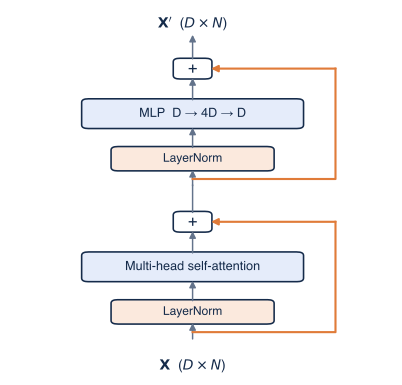
Figure 12.3 A transformer layer (pre-norm). The input is a $D \times N$ matrix, one column per token. The first block normalizes each column, applies multi-head self-attention across all columns and adds the result back (orange: residual connection). The second block normalizes each column, applies the same two-layer MLP to every column separately and adds the result back. The output has the same shape as the input, so layers can be stacked.

Counting a real model

A transformer stacks such layers between the input embeddings and an output layer. For GPT-2 small [6], with $D = 768$, 12 layers, 12 heads and a context of 1,024 tokens, the parameters are:

Component	Parameters
Multi-head self-attention, per layer ($4D^2 + 4D$)	2,362,368
MLP, per layer ($8D^2 + 5D$)	4,722,432
Two layer norms, per layer ($4D$)	3,072
One transformer layer	7,087,872
12 layers	85,054,464
Token embeddings ($50{,}257 \times 768$)	38,597,376
Position embeddings ($1{,}024 \times 768$)	786,432
Final layer norm	1,536
Total	124,439,808

The output layer that turns each final vector into scores over the vocabulary reuses the token embedding matrix, a common choice called weight tying, so it adds no parameters. Each layer has about $12D^2$ parameters, two thirds of them in the MLP. The embeddings take almost a third of this small model, a share that shrinks as $D$ and the number of layers grow.

The computation per token follows the same pattern. Each parameter in a matrix product is used once per token, so the forward pass needs about one multiply-add per parameter per token, plus the attention terms $2ND$ per layer. For GPT-2 small with $N = 1{,}024$, that is about 142 million multiply-adds per token.

8. Encoders, decoders and masks

Transformers are used in three configurations, which differ in which positions may attend to which.

Encoders let every position attend to every other, as in sections 2–7, and produce one output vector per token that summarizes the token in its full context. BERT [5] is the standard example. It is trained by hiding about 15% of the tokens of a text and predicting them from the rest, a task called masked language modelling, and its outputs are then used for tasks such as classifying sentences or finding answers in a passage.

Decoders generate text one token at a time, and a position may attend only to itself and earlier positions. This is enforced by a causal mask: before the softmax, every score $s_{mn}$ with $m > n$ is set to $-\infty$, so its weight becomes zero. In the example of section 2 (figure 12.1c), the first position can attend only to itself, so its weight is 1; the second splits its weight over positions 1 and 2 in the ratio of $e^0$ to $e^2$, giving $(0.119, 0.881)$; the third is unchanged. A decoder is trained to predict the next token at every position: the output at position $n$, after a final layer that produces one score per vocabulary token, should give high probability to token $n + 1$. The loss is the cross-entropy of article 4, averaged over positions. Because of the mask, the output at position $n$ never sees token $n + 1$, so all $N$ predictions of a text can be trained at once from a single forward pass. GPT-2 and most large language models (as of 2026) are decoders.

To generate, a decoder computes the scores for the next token, samples one, appends it to the input and repeats. The keys and values of earlier positions do not change when a token is appended, so they are stored (the KV cache), and each new token costs one column of queries, keys and values plus attention over the $N$ stored positions, rather than recomputing the whole sequence.

Encoder–decoders combine the two, for tasks that map one sequence to another, such as translation. The original transformer [2] was of this kind. The decoder layers contain an extra cross-attention block in which the queries come from the decoder and the keys and values from the encoder's outputs, so that each generated token can consult the whole input sentence.

9. Beyond text

Nothing in a transformer layer is specific to language: it processes a set of vectors, with positions supplied by the encodings. The vision transformer [8] cuts a $224 \times 224$ color image into $16 \times 16$ patches, giving 196 patches of $16 \times 16 \times 3 = 768$ values; a linear map turns each patch into a token, and a standard encoder processes the 196 tokens. Without the locality and weight sharing of convolutions (article 10), it needs more training data or stronger augmentation to reach the same accuracy, but it scales well when data are plentiful. The same recipe, turning the input into tokens and adding positions, has been applied to audio, protein sequences, video and combinations of them.

10. What attention does and does not tell us

Attention weights are easy to visualize, and it is tempting to read them as explanations: "the model looked at this word". That reading needs care. Each layer has many heads, outputs pass through MLPs and residual paths that attention weights do not show, and later layers attend to vectors that already mix information from many positions. Jain and Wallace [11] found that quite different attention weights can produce the same predictions. Attention weights describe how one layer mixes its inputs, not why the model produced its output.

The quadratic cost of section 3 is the main practical limit. For a context of 8,192 tokens, each head of each layer computes about 67 million scores. Exact attention can be computed without storing the full $N \times N$ matrix, by processing it in blocks that fit in fast memory [14], and many approximations reduce the cost further; but the computation of exact attention still grows with $N^2$.

Summary

A text is split into tokens, each mapped to a learned embedding, giving one vector per position. Self-attention lets every position compute a query, compare it with every position's key, turn the scores into weights with a softmax, and take the weighted average of the values. The layer accepts any length with the same parameters, is equivariant to reordering, and costs time and memory that grow with the square of the length. Dividing the scores by $\sqrt{D_q}$ keeps the softmax from saturating, positional encodings restore the order that attention ignores, and multiple heads let a layer attend in several ways at once. A transformer layer combines multi-head attention with a per-position MLP, each inside a residual connection with layer normalization; GPT-2 small stacks twelve of them for 124 million parameters. Encoders attend in both directions, decoders use a causal mask and are trained to predict the next token, and encoder–decoders connect the two with cross-attention.

This completes part 2. Article 7 showed why depth helps, and article 8 how all of a deep network's gradients are computed. Article 9 explained how to keep large networks from fitting noise, and article 10 how to build knowledge about images into the architecture. Article 11 made very deep networks trainable, and article 12 combined these pieces into the architecture behind today's language models.

Notes

History. Attention was introduced for machine translation by Bahdanau, Cho and Bengio [3] in 2014–15, as a way for a recurrent decoder to look back at the encoded source sentence. Vaswani and colleagues [2] showed in 2017 that attention without recurrence suffices, and named the result the transformer. Its encoder–decoder base model had 6 layers in each half, $D = 512$ and 8 heads.

Scaling. Kaplan and colleagues [12] found that the loss of language models falls smoothly, approximately as a power law, as parameters, data and computation grow together, over many orders of magnitude. Hoffmann and colleagues [13] found that for a fixed computational budget, the number of training tokens should grow in proportion to the number of parameters, about 20 tokens per parameter in their experiments. These are empirical regularities, not laws of nature, and their exponents depend on the data and architecture. GPT-3 [15], in 2020, had 175 billion parameters in 96 layers with $D = 12{,}288$; the transformer layer itself is little changed since 2017.

Efficient attention. Approaches to the quadratic cost include attending only within local windows, to a fixed set of global tokens, or through low-rank approximations of the attention matrix, as well as architectures that replace attention with recurrences that can be trained in parallel. Exact attention with careful memory management [14] remains the most common choice at moderate lengths.

Reading further. Chapter 12 of Understanding Deep Learning [1] covers transformers, including the matrix formulation used here, encoders, decoders and the vision transformer.

Problems

Problem 12.1 In the example of section 2, compute the output for position 2 by hand. (Answer: $0.063\,(1, 0) + 0.468\,(0, 1) + 0.468\,(1, 1) = (0.532, 0.937)$.)

Problem 12.2 How many parameters does a single-head self-attention layer have with $D = 512$ and $D_q = 64$, including biases? How does the number change if the sequence length doubles? (Answer: $2 \times 64 \times 512 + 512^2 + 2 \times 64 + 512 = 328{,}320$; it does not change.)

Problem 12.3 A query and a key have 128 independent elements with mean 0 and variance 1. What is the standard deviation of their dot product, before and after scaling? (Answer: $\sqrt{128} \approx 11.3$ before, 1 after.)

Problem 12.4 Use $\mathbf{R}(\alpha)^\top\mathbf{R}(\beta) = \mathbf{R}(\beta - \alpha)$ to verify equation 12.7. Then show that shifting both positions by the same amount leaves the score unchanged. (Hint: replace $m$ and $n$ by $m + c$ and $n + c$; the difference is unchanged.)

Problem 12.5 Apply a causal mask to the scores of the third query in section 2, $(1, 4, 5)$. Does the result change? Why? (Answer: no; the third position may attend to positions 1–3, which is all of them, so the weights stay $(0.013, 0.265, 0.721)$.)

Problem 12.6 Using the per-layer count $12D^2 + 13D$, how many parameters do the 24 transformer layers of a model with $D = 1{,}024$ have? (Answer: $24 \times (12 \times 1{,}048{,}576 + 13{,}312) = 302{,}309{,}376$, about 302 million.)

Problem 12.7 A vision transformer uses $14 \times 14$ patches on a $224 \times 224$ image. How many tokens does it process, and by what factor does the attention cost grow compared with $16 \times 16$ patches? (Answer: $16^2 = 256$ tokens; the cost grows by $(256/196)^2 \approx 1.71$.)

References

• 1: Simon J.D. Prince (2023). Understanding Deep Learning. MIT Press.
• 2: Ashish Vaswani, Noam Shazeer, Niki Parmar, Jakob Uszkoreit, Llion Jones, Aidan Gomez, Łukasz Kaiser and Illia Polosukhin (2017). Attention is all you need. Advances in Neural Information Processing Systems 30.
• 3: Dzmitry Bahdanau, Kyunghyun Cho and Yoshua Bengio (2015). Neural machine translation by jointly learning to align and translate. International Conference on Learning Representations.
• 4: Rico Sennrich, Barry Haddow and Alexandra Birch (2016). Neural machine translation of rare words with subword units. Annual Meeting of the Association for Computational Linguistics.
• 5: Jacob Devlin, Ming-Wei Chang, Kenton Lee and Kristina Toutanova (2019). BERT: pre-training of deep bidirectional transformers for language understanding. Conference of the North American Chapter of the Association for Computational Linguistics.
• 6: Alec Radford, Jeffrey Wu, Rewon Child, David Luan, Dario Amodei and Ilya Sutskever (2019). Language models are unsupervised multitask learners. OpenAI technical report.
• 7: Jianlin Su, Murtadha Ahmed, Yu Lu, Shengfeng Pan, Wen Bo and Yunfeng Liu (2024). RoFormer: enhanced transformer with rotary position embedding. Neurocomputing 568.
• 8: Alexey Dosovitskiy, Lucas Beyer, Alexander Kolesnikov, Dirk Weissenborn, Xiaohua Zhai, Thomas Unterthiner, Mostafa Dehghani, Matthias Minderer, Georg Heigold, Sylvain Gelly, Jakob Uszkoreit and Neil Houlsby (2021). An image is worth 16x16 words: transformers for image recognition at scale. International Conference on Learning Representations.
• 9: Ruibin Xiong, Yunchang Yang, Di He, Kai Zheng, Shuxin Zheng, Chen Xing, Huishuai Zhang, Yanyan Lan, Liwei Wang and Tie-Yan Liu (2020). On layer normalization in the transformer architecture. International Conference on Machine Learning.
• 10: Dan Hendrycks and Kevin Gimpel (2016). Gaussian error linear units (GELUs). arXiv:1606.08415.
• 11: Sarthak Jain and Byron Wallace (2019). Attention is not explanation. Conference of the North American Chapter of the Association for Computational Linguistics.
• 12: Jared Kaplan, Sam McCandlish, Tom Henighan, Tom Brown, Benjamin Chess, Rewon Child, Scott Gray, Alec Radford, Jeffrey Wu and Dario Amodei (2020). Scaling laws for neural language models. arXiv:2001.08361.
• 13: Jordan Hoffmann, Sebastian Borgeaud, Arthur Mensch and colleagues (2022). Training compute-optimal large language models. Advances in Neural Information Processing Systems 35.
• 14: Tri Dao, Daniel Fu, Stefano Ermon, Atri Rudra and Christopher Ré (2022). FlashAttention: fast and memory-efficient exact attention with IO-awareness. Advances in Neural Information Processing Systems 35.
• 15: Tom Brown, Benjamin Mann, Nick Ryder, Melanie Subbiah and colleagues (2020). Language models are few-shot learners. Advances in Neural Information Processing Systems 33.