Tensor shapes, parameter counts and computational cost

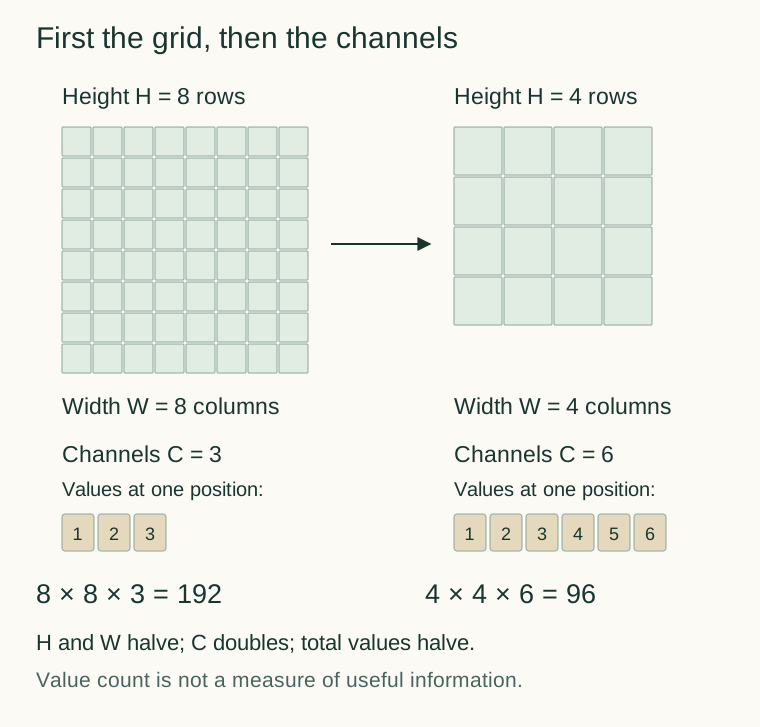
A shape calculation answers practical design questions before a layer is run: whether two blocks can connect, how much activation storage is needed, and how much arithmetic a convolution requires. Naming the axes first turns a change such as eight-by-eight-by-three to four-by-four-by-six into several measurable decisions rather than one vague change in dimension.

A tensor shape records the sizes of named axes. It does not by itself specify the number of trainable parameters, the computational cost or the information preserved by a transformation. These quantities require separate definitions and calculations.

1. Axes, vector dimension and matrix rank

For a channels-last image, $(H,W,C)$ denotes height, width and channel count. A batch has shape $(N,H,W,C)$, whereas the channels-first convention is $(N,C,H,W)$. Axis meanings cannot be recovered reliably from an unlabeled list of numbers.

The number of tensor axes is sometimes called tensor rank in array libraries. This differs from matrix rank, which counts linearly independent columns. Vector dimension instead counts coordinates in a vector. The term “dimension” must therefore be interpreted in its stated context.

An image of shape $(8,8,3)$ contains $8\cdot8\cdot3=192$ scalar entries. Flattening gives a vector in $\mathbb R^{192}$ without discarding entries if their order is preserved. Entry count alone, however, is not a measure of information content.

2. Derivation of convolution output size

Consider an input axis of length $H$, symmetric padding $p$, kernel length $k$, dilation $D$ and stride $s$. Assume positive integer $k,D,s$ and nonnegative integer $p$. The span from the first to the last kernel sample gives the effective kernel size:

$$k_{\mathrm{eff}}=D(k-1)+1$$

In the padded input, window starts are $0,s,2s,\ldots,qs$. The last window fits when $qs+k_{\mathrm{eff}}\le H+2p$. The number of valid starts is consequently:

$$H_{\mathrm{out}}=\left\lfloor\frac{H+2p-D(k-1)-1}{s}\right\rfloor+1$$

The same argument applies to width. At least one window must fit; asymmetric padding replaces $2p$ with the sum of the two padding amounts. The floor cannot be omitted when the available span is not divisible by the stride. [1]

3. Activations, parameters and operations

For $H=W=8$, $C_{\mathrm{in}}=3$, $C_{\mathrm{out}}=6$, $k=3$, $p=1$, $s=2$ and $D=1$:

$$H_{\mathrm{out}}=W_{\mathrm{out}}=\lfloor7/2\rfloor+1=4$$

The transformation is $(8,8,3)\to(4,4,6)$: height and width halve, while channel count doubles. Each sample has 192 input entries and 96 output entries. Including one bias per output channel, the shared parameter count is:

$$P=3\cdot3\cdot3\cdot6+6=168$$

Counting one multiply–accumulate (MAC) for each kernel coefficient at each output position, and excluding bias additions, gives:

$$\mathrm{MACs}=4\cdot4\cdot6\cdot3\cdot3\cdot3=2592$$

A batch of size $N$ multiplies the activation count and MAC count by $N$, but leaves the parameter count at 168. The operation-counting convention matters: one MAC may be reported as two floating-point operations.

4. Grouped and depthwise convolution

For $g$ groups, both input and output channel counts must be divisible by $g$. Each output channel accesses $C_{\mathrm{in}}/g$ input channels, yielding:

$$P_g=k_hk_w\frac{C_{\mathrm{in}}C_{\mathrm{out}}}{g}+C_{\mathrm{out}}$$

Depthwise convolution corresponds to $g=C_{\mathrm{in}}$, with $C_{\mathrm{out}}$ an integer multiple of $C_{\mathrm{in}}$. Grouping restricts channel connectivity; the lower count does not preserve every interaction available in an ordinary dense convolution. [1]

5. Receptive-field span

Let $r_l$ denote the theoretical receptive-field span at layer $l$, and $j_l$ the spacing between neighboring outputs measured in original input coordinates. Starting from $r_0=j_0=1$:

$$r_l=r_{l-1}+(k_l-1)D_lj_{l-1},\qquad j_l=s_lj_{l-1}$$

The additional span contains $(k_l-1)D_l$ gaps, each of size $j_{l-1}$. For two kernel-size-three layers with dilation one and strides two then one, the results are $(r_1,j_1)=(3,2)$ and $(r_2,j_2)=(7,2)$.

The span describes a possible input dependency, not equal influence from every position. Padding also requires distinguishing original data from extended coordinates at boundaries. A complete shape analysis therefore states the changing axes, activation and parameter counts, operation count, and possible spatial dependencies separately. [2]

References

• 1: PyTorch Conv2d
• 2: Dive into Deep Learning: Padding and Stride