Convolution and directional edge responses

An edge is associated with a change across neighboring values. Subtracting one side of a neighborhood from the other suppresses a uniform region and produces a response at a transition. A convolution kernel encodes this comparison as a small table of weights, so the relation between its coefficients and its behavior can be calculated exactly.

A local linear filter computes a weighted sum over neighboring values. Its response depends on the coefficient pattern, spatial direction, boundary treatment and numerical scale. A fixed edge detector provides an explicit example of this operation before its coefficients are made trainable in a convolutional network.

1. Cross-correlation and convolution

For a single-channel input $X$ and a $3\times3$ kernel $K$ indexed around its center, cross-correlation is:

$$Y_{i,j}=\sum_{u=-1}^{1}\sum_{v=-1}^{1}K_{u,v}X_{i+u,j+v}$$

Mathematical convolution instead reverses the spatial offsets:

$$(K*X)_{i,j}=\sum_{u=-1}^{1}\sum_{v=-1}^{1}K_{u,v}X_{i-u,j-v}$$

Equivalently, convolution can be implemented as cross-correlation with a spatially flipped kernel. Many neural-network libraries call the unflipped operation convolution; the convention must therefore be specified before comparing coefficients or response signs. [1]

The numerical example below uses cross-correlation, stride one and one-pixel replicate padding. Replicate padding extends the nearest boundary value. These choices preserve the input's spatial size and fully determine the computation at its edges.

2. A directional Sobel operator

The horizontal Sobel kernel is:

$$K_x=\begin{bmatrix}-1&0&1\\-2&0&2\\-1&0&1\end{bmatrix} =\begin{bmatrix}1\\2\\1\end{bmatrix} \begin{bmatrix}-1&0&1\end{bmatrix}$$

Its factorization combines a horizontal difference with a vertical weighted sum. The coefficients sum to zero, so a constant patch produces zero response. For a horizontal ramp $X_{i,j}=aj+b$, each row's difference is $2a$; weighting the three rows by $1,2,1$ gives:

$$G_x=8a$$

For unit grid spacing, division by eight therefore returns the slope of this particular ramp. The unnormalized operator has a scale factor, which matters when interpreting magnitudes. Its response is strong for a vertical boundary because the intensity changes along the horizontal coordinate. [2]

3. A complete local calculation

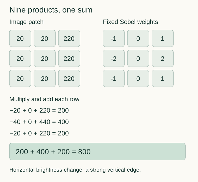
Consider the patch:

$$P=\begin{bmatrix}20&20&220\\20&20&220\\20&20&220\end{bmatrix}$$

Multiplying corresponding entries and summing gives:

$$G_x=(-20+220)+(-40+440)+(-20+220)=800$$

The middle row contributes twice as much because its nonzero weights have magnitude two. Reversing the intensity transition reverses the response sign to $-800$. This sign distinguishes transition direction; the absolute magnitude alone does not retain that distinction.

4. Numerical input and response visualization

The test input has height 128 and width 192. Its value is 220 for coordinates $48\le x\le143$, $32\le y\le95$, and 20 elsewhere. The patch centered at $(x,y)=(47,50)$ is exactly the patch used above. These values define a synthetic numerical input, rather than an observed model output.

For this input, the maximum absolute horizontal response is 800. The displayed image is computed using:

$$D_{i,j}=\operatorname{round}\left(255\frac{|G_x(i,j)|}{800}\right)$$

The denominator 800 is specific to this input. For arbitrary values between zero and 255, the sum of positive kernel weights is four, giving a maximum possible absolute response of $4\cdot255=1020$. Display normalization should not be confused with the filter's raw numerical output.

5. Direction and interpretation

The vertical operator is $K_y=K_x^\top$. A two-direction gradient magnitude can be formed as $\sqrt{G_x^2+G_y^2}$, but the image above displays only $|G_x|$. A zero horizontal response is therefore not evidence that no boundary exists; a horizontal boundary may respond to the other operator.

Nor does a large response establish an object's identity. The filter measures a local directional variation according to fixed coefficients. In a CNN, coefficients can instead be fitted to a task, while the underlying sliding weighted-sum computation remains available as a building block. [2]

References

• 1: Dive into Deep Learning, Convolutions for Images
• 2: OpenCV, Sobel Derivatives