Language models: probability, training and generation

Generating a sentence requires choosing among possible continuations at each step. A probability distribution expresses how the model ranks those alternatives; training changes that distribution so observed continuations receive greater probability. This connects the next-token objective to the repeated computation that produces a complete answer.

An autoregressive language model defines conditional probabilities over discrete token sequences. Training estimates its parameters from observed sequences; generation selects successive tokens from the resulting distributions. These operations share a probability model but differ in both their inputs and their effects on the parameters.

1. Sequence probability

Let $\mathcal V$ be the vocabulary, $V=|\mathcal V|$ its size, and $x_{1:T}=(x_1,\ldots,x_T)$ a sequence. The probability chain rule gives:

$$p_\theta(x_{1:T}) =\prod_{t=1}^{T}p_\theta(x_t\mid x_{<t}), \qquad x_{<t}=(x_1,\ldots,x_{t-1})$$

The first factor is conditioned on an empty prefix or an explicitly specified start token. For conditional generation, the supplied prompt forms part of the prefix. An end token can represent termination within the probability model. [1]

The factorization follows from conditional probability and permits dependence between positions. A Transformer can parameterize the conditional distributions. With a finite context limit $C$, each computation uses the prefix admitted by that configuration.

2. From hidden states to probabilities

Suppose $h_t\in\mathbb R^d$ is the final hidden vector used to predict $x_t$ from its prefix. The output projection produces a vector of unnormalized scores, or logits:

$$z_t=Uh_t+b,\qquad U\in\mathbb R^{V\times d},\quad b\in\mathbb R^V$$

Softmax converts these scores into probabilities:

$$p_{t,k}=\frac{e^{z_{t,k}}}{\sum_{j=1}^{V}e^{z_{t,j}}}$$

For finite logits, each probability is positive and their sum is one. Direct exponentiation can overflow numerically. Subtracting the largest logit, $m_t=\max_jz_{t,j}$, yields the equivalent expression:

$$p_{t,k}=\frac{e^{z_{t,k}-m_t}}{\sum_j e^{z_{t,j}-m_t}}$$

The factor $e^{-m_t}$ cancels between numerator and denominator. This transformation improves numerical evaluation without changing the represented distribution. [2]

3. Training objective and gradient

Maximum-likelihood training maximizes the probability assigned to observed sequences. Taking the negative logarithm converts a product into a sum. A token-average objective for one sequence is:

$$\mathcal L(\theta) =-\frac1T\sum_{t=1}^{T}\log p_\theta(x_t\mid x_{<t})$$

Averaging over tokens and averaging per-sequence losses produce different sample weights when sequence lengths vary. During next-token training, the observed prefix supplies the condition and the observed next token supplies the target. Causal attention excludes future positions from the computation used to predict a target. [3]

At a single position with target index $y$, the negative log-likelihood expands to:

$$\ell=-z_y+\log\sum_j e^{z_j}$$

Differentiating the linear term and the log-sum-exp term gives:

$$\frac{\partial\ell}{\partial z_k} =-\mathbf1[k=y]+\frac{e^{z_k}}{\sum_j e^{z_j}} =p_k-\mathbf1[k=y]$$

Here $\mathbf1[k=y]$ equals one for the target class and zero otherwise. This is the derivative with respect to a logit. Parameter gradients additionally require the chain rule through the output projection and preceding layers.

4. A numerical example

For a constructed three-token vocabulary, let $z=(\log2,0,0)$. Exponentiation gives $(2,1,1)$, so normalization gives:

$$p=(1/2,1/4,1/4)$$

When the first token is the target, the loss is $\ell=\log2\approx0.693147$, and:

$$\nabla_z\ell=(-1/2,1/4,1/4)$$

The calculation concerns token occurrence under a particular context. The first probability of $1/2$ therefore describes a possible continuation, not the factual correctness of a statement.

5. Generation and decoding

Decoding may select the most probable token, $\arg\max_k p_k$, or sample from the distribution. A positive temperature $\tau$ modifies sampling probabilities through $\operatorname{softmax}(z/\tau)$. For the example above, $\tau=2$ changes the first probability to $\sqrt2/(\sqrt2+2)\approx0.414214$.

The selected token is appended to the prefix, and the computation repeats until a stopping condition is reached. During ordinary inference, $\theta$ remains fixed. A new prefix changes the conditional distribution without performing a training update. External storage, retrieval and subsequent training are separate system operations.

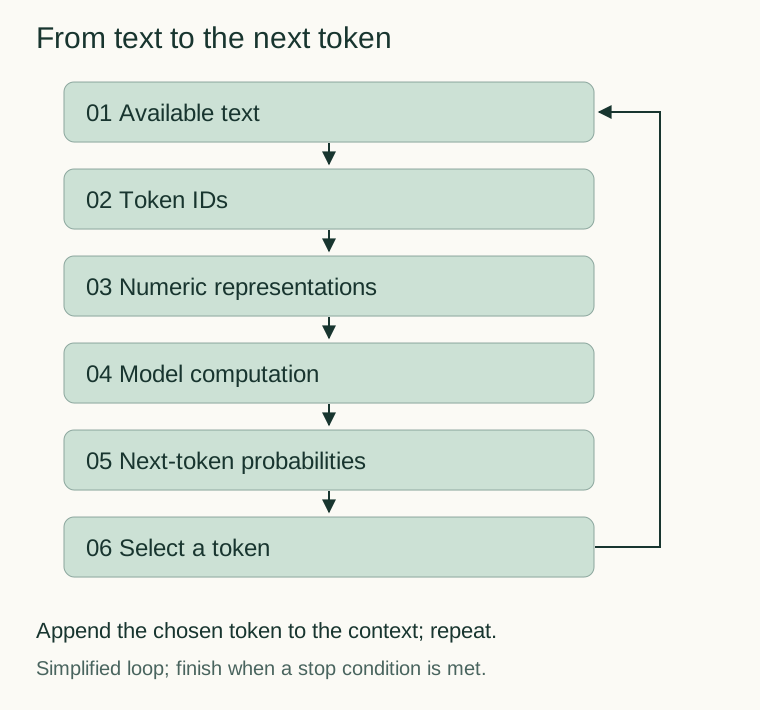
The diagram describes the computational order. The equations specify the distribution, training objective and distinction between inference and parameter updates. [3]

References

• 1: Dive into Deep Learning, Language Models
• 2: Dive into Deep Learning, Softmax Regression
• 3: Attention Is All You Need